Catching AI with its pants down: Optimize an Artificial Neuron from Scratch

We will strip the mighty, massively hyped, highly dignified AI of its cloths, and bring its innermost details down to earth!

• Prologue
  • Notation for tensors
• Gradient Descent Algorithm
• Chain rule for cost gradients
  • Cost gradient with respect to weights
    • Preactivation gradient with respect to weights
    • Activation gradient with respect to preactivations
    • Cost gradient with respect to activations
    • Consolidate the results
  • Cost gradient with respect to biases

Prologue

This is part 3 of the blog series, Catching AI with its pants down. This blog series aims to explore the inner workings of neural networks and show how to build a standard feedforward neural network from scratch.

In this part, I will dive into the mathematical details of training (optimizing) an artificial neuron via gradient descent. This will be a math-heavy article, so get your pen and scratch papers ready. But I made sure to simplify things.

Parts	The complete index for Catching AI with its pants down
Pant 1	Some Musings About AI
Pant 2	Understand an Artificial Neuron from Scratch
Pant 3	Optimize an Artificial Neuron from Scratch
Pant 4	Implement an Artificial Neuron from Scratch
Pant 5	Understand a Neural Network from Scratch
Pant 6	Optimize a Neural Network from Scratch
Pant 7	Implement a Neural Network from Scratch
Pant 8	Demonstration of the Models in Action

Let’s recap before we begin the last dash:

Recall that an artificial neuron can be succinctly described as a function that takes in $ \mathbf{X} $ and uses its parameters $ \vec{w} $ to do some computations to spit out an activation value that we expect to be close to the actual correct value (the ground truth), $ \vec{y} $. This also means that we expect some level of error between the activation value and the ground truth, and the loss function gives us a measure of this error in the form of single scalar value, the loss (or cost).

We want the activation to be as close as possible to the ground truth by getting the loss to be as small as possible. In order to do that, we want to find a set of values for $ \vec{w} $ such that the loss is always as low as possible.

What remains to be seen is how we find this $ \vec{w} $ that minimizes the loss.

Notation for tensors

Just like in every article for this blog series, unless explicitly started otherwise, matrices (and higher-order tensors, which should be rare in this blog series) are denoted with boldfaced, non-italic, uppercase letters; vectors are denoted with non-boldfaced, italic letters accented with a right arrow; and scalars are denoted with non-boldfaced, italic letters. E.g. \(\mathbf{A}\) is a matrix, \(\vec{a}\) is a vector, and \(a\) or \(A\) is a scalar.

Gradient Descent Algorithm

As we saw in part 2, we have a loss function that is a function of the weights and biases, and we need a way to find the set of weights and biases that minimizes the loss. This is a clearcut optimization problem.

There are many ways to solve this optimization problem, but we will go with the one that scales excellently with deep neural networks, since that is the eventual goal of this writeup. And that brings us to the gradient descent algorithm. A method for finding local extrema of a function using the gradient of that function. It was introduced in 1847 by Augustin-Louis Cauchy, and still remains widely used in deep learning today.

We will illustrate how it works using a simple scenario where we have a dataset made of one feature and one target, and we want to use the mean squared error as cost function. We specify a linear activation function (\(a=f(a)\)) for the neuron. Then the equation for our neuron will be:

\[a=f\left(z\right)=w_1\ \cdot x_1+w_0\]

Our cost function becomes:

\[J=\frac{1}{m}\cdot\sum_{j=0}^{m}{({y}_j-a_j)}^2=\frac{1}{m}\cdot\sum_{j=0}^{m}{(y_j-\ w_{1,j}\ \cdot x_{1,j}+w_{0,j})}^2\]

Let’s further simplify our scenario by assuming we will only run computations for only one datapoint at a time.

\[J={(y_j-\ w_{1,j}\ \cdot x_{1,j}+w_{0,j})}^2\]

If we hold \(y_j\) and \(x_{1,j}\) constant, which is logical since they come directly from data, we observe that our cost is a function of just the parameters \(w_0\) and \(w_1\). And we can easily plot the curve.

Plot of cost against two parameters.

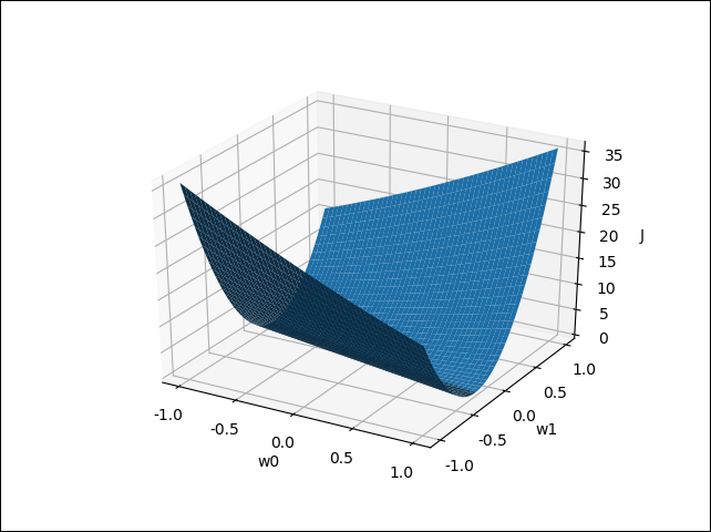
From the plot we can easily see what values we can set \(w_0\) and \(w_1\) to in order to produce the most minimal cost. Any picks for \(w_0\) and \(w_1\) from the bottom of the valley will give a minimal cost.

The gradient descent algorithm formalizes the idea we just followed. It pretty much says: Start somewhere on the cost function (in this case, the plotted surface) and only take steps in the direction of negative gradient (i.e. direction of descent). Once you hit a minimum, any step you take will always turn out to be in the direction of ascent and therefore the iteration will no longer improve the minimization of the cost.

In mathematical terms, it is this:

\[w_{new}=w_{old}-\gamma\frac{\partial J}{\partial w_{old}}\] \[b_{new}=b_{old}-\gamma\frac{\partial J}{\partial b_{old}}\]

Where $ \gamma $ is the step size (a.k.a. learning rate).

The above equations are used in updating the parameters at the end of each round or iteration of training. The equations are applied to each of the parameters in the model (the artificial neuron). For instance, for our toy dataset, there would be two weights, one for each feature (input variable) of the dataset, and one bias for the bias node. All three parameters will be updated using the equations. That marks the end of one round or iteration of training.

Stochastic gradient descent means that randomization is introduced during the selection of the batch of datapoints to be used in the calculations of the gradient descent. Some people will distinguish further by defining mini-batch stochastic gradient descent as when a batch of datapoints is randomly selected from the dataset and used, while stochastic gradient descent refers to just using a single randomly selected datapoint for each entire round of computations.

If we had more than two parameters, or a non-linear activation function, or some other property that makes our neuron more complicated, using a plot to find the parameters that minimize the error becomes just impractical. We must use the mathematical formulation.

What remains to be answered is how we can efficiently compute \(\frac{\partial J}{\partial w_{old}}\) and \(\frac{\partial J}{\partial b_{old}}\).

Chain rule for cost gradients

Heads up: For this part, which is the real meat of the training process, I advise that you bring out a pen and some paper to work along if this is your first time working with Jacobians.

Let’s focus on just \(\frac{\partial J}{\partial \vec{w}}\) for now. To compute the cost gradient \(\frac{\partial J}{\partial \vec{w}}\) we simply use the chain rule.

Cost gradient with respect to weights

\[\frac{\partial J}{\partial \vec{w}}=\ \frac{\partial J}{\partial \vec{a}}\frac{\partial \vec{a}}{\partial \vec{z}}\frac{\partial \vec{z}}{\partial \vec{w}}\]

The gradient \(\frac{\partial J}{\partial \vec{a}}\) (it is also a Jacobian) depends on the choice of the cost function because we can’t do anything if we haven’t picked what function to use for \(J\). Also, \(\frac{\partial \vec{a}}{\partial \vec{z}}\) depends on the choice of activation function, although we can solve it for an arbitrary function.

But for \(\frac{\partial \vec{z}}{\partial \vec{w}}\), we know that preactivation (\(\vec{z}\)), at least for one neuron, will always be a simple linear combination of the parameters and the input data (see part 2):

\[\vec{z}=\vec{w}\mathbf{X}+\vec{b}\]

This is also always true in standard feedforward neural networks (a.k.a. multilayer perceptron), but not so for every flavour of neural networks (e.g. convolutional neural networks have a convolution operation instead of a multiplication between \(\vec{w}\) and \(\mathbf{X}\)).

Before we move any further, it’s important you understand what Jacobians are. In a nutshell, the Jacobian of a vector-valued function (a function that returns a vector), which is what we are working with here, is a matrix that contains all of the function’s first order partial derivatives. It is the way to properly characterize the partial derivatives of a vector function with respect to all its input variables.

If you were not already familiar with Jacobians or still unclear of what it is, I found this video that should help (or just search for “Jacobian matrix” on YouTube and you’ll see many great introductory videos).

Our Jacobians in matrix representation are as follows:

\[\frac{\partial J}{\partial \vec{w}}=\left[\begin{matrix}\frac{\partial J}{\partial w_1}&\frac{\partial J}{\partial w_2}&\cdots&\frac{\partial J}{\partial w_n}\\\end{matrix}\right]\] \[\frac{\partial J}{\partial \vec{a}}=\left[\begin{matrix}\frac{\partial J}{\partial a_1}&\frac{\partial J}{\partial a_2}&\cdots&\frac{\partial J}{\partial a_m}\\\end{matrix}\right]\] \[\frac{\partial \vec{a}}{\partial \vec{z}}=\left[\begin{matrix}\frac{\partial a_1}{\partial z_1}&\frac{\partial a_1}{\partial z_2}&\cdots&\frac{\partial a_1}{\partial z_m}\\\frac{\partial a_2}{\partial z_1}&\frac{\partial a_2}{\partial z_2}&\cdots&\frac{\partial a_2}{\partial z_m}\\\vdots&\vdots&\ddots&\vdots\\\frac{\partial a_m}{\partial z_1}&\frac{\partial a_m}{\partial z_2}&\cdots&\frac{\partial a_m}{\partial z_m}\\\end{matrix}\right]\] \[\frac{\partial \vec{z}}{\partial \vec{w}}=\left[\begin{matrix}\frac{\partial z_1}{\partial w_1}&\frac{\partial z_1}{\partial w_2}&\cdots&\frac{\partial z_1}{\partial w_n}\\\frac{\partial z_2}{\partial w_1}&\frac{\partial z_2}{\partial w_2}&\cdots&\frac{\partial z_2}{\partial w_n}\\\vdots&\vdots&\ddots&\vdots\\\frac{\partial z_m}{\partial w_1}&\frac{\partial z_m}{\partial w_2}&\cdots&\frac{\partial z_m}{\partial w_n}\\\end{matrix}\right]\]

Where their shapes are: $ \frac{\partial J}{\partial \vec{w}} $ is $ 1 $-by-$ n $, $ \frac{\partial J}{\partial \vec{a}} $ is $ 1 $-by-$ m $, $ \frac{\partial \vec{a}}{\partial \vec{z}} $ is $ m $-by-$ m $, and $ \frac{\partial \vec{z}}{\partial \vec{w}} $ is $ m $-by-$ n $.

The shapes show us that matrix multiplications present in the chain rule expansion are valid.

Preactivation gradient with respect to weights

From the equation for \(\vec{z}\) stated above, we can immediately compute the Jacobian \(\frac{\partial \vec{z}}{\partial \vec{w}}\).

We can observe that the Jacobian \(\frac{\partial \vec{z}}{\partial \vec{w}}\) is an \(m\)-by-\(n\) matrix. But at this stage, our Jacobian hasn’t given us anything useful because we still need the solution for each scalar element of the matrix.

We’ll solve an arbitrary element of the Jacobian and extend the pattern to the rest. Let’s begin.

We pick an arbitrary scalar element \(\frac{\partial z_j}{\partial w_i}\) from the matrix, and immediately we observe that we have already encountered the generalized elements \(z_j\) and \(w_i\) in the following equation:

\[z_j=w_1\ \cdot x_{1,j}+w_2\ \cdot x_{2,j}+\ldots+w_n\ \cdot x_{n,j}+w_0=\sum_{i=0}^{n}{w_i\ \cdot x_{i,j}}\]

Therefore:

\[\frac{\partial z_j}{\partial w_i}=\frac{\partial\left(\sum_{i=0}^{n}{w_i\ \cdot x_{i,j}}\right)}{\partial w_i}\]

The above is a partial derivative w.r.t. \(w_i\), so we temporarily consider \(x_{i,j}\) to be a constant.

\[\frac{\partial z_j}{\partial w_i}=\frac{\partial\left(\sum_{i=0}^{n}{w_i\ \cdot x_{i,j}}\right)}{\partial w_i}=x_{i,j}\]

(If it’s unclear how the above worked out, expand out the summation and do the derivatives term by term, and keep in mind that \(x_{i,j}\) is considered to be constant, because this is a partial differentiation w.r.t. \(w_i\)).

We substitute the result back into the Jacobian:

\[\frac{\partial \vec{z}}{\partial \vec{w}}=\left[\begin{matrix}x_{1,1}&x_{2,1}&\cdots&x_{n,1}\\x_{1,2}&x_{2,2}&\cdots&x_{n,2}\\\vdots&\vdots&\ddots&\vdots\\x_{1,m}&x_{2,m}&\cdots&x_{n,m}\\\end{matrix}\right]\]

Recall that we originally defined \(\mathbf{X}\) as:

\[\mathbf{X}=\left[\begin{matrix}x_{1,1}&x_{1,2}&\cdots&x_{1,m}\\x_{2,1}&x_{2,2}&\cdots&x_{2,m}\\\vdots&\vdots&\ddots&\vdots\\x_{n,1}&x_{n,2}&\cdots&x_{n,m}\\\end{matrix}\right]\]

Therefore, we observe that \(\frac{\partial \vec{z}}{\partial \vec{w}}\) is exactly the transpose of our original definition of \(\mathbf{X}\):

\[\frac{\partial \vec{z}}{\partial \vec{w}}= \mathbf{X}^T\]

One Jacobian is down. Two more to go.

Activation gradient with respect to preactivations

The Jacobian \(\frac{\partial \vec{a}}{\partial \vec{z}}\) depends on the choice of activation function, since it is obviously the gradient of the activation w.r.t. to preactivation (i.e. the derivative of the activation function). We cannot characterize it until we fully characterize the equation for \(\vec{a}\).

Let’s go with the logistic activation function:

\[\vec{a}=\frac{1}{1+e^{-\vec{z}}}\] \[\frac{\partial \vec{a}}{\partial \vec{z}}=\left[\begin{matrix}\frac{\partial a_1}{\partial z_1}&\frac{\partial a_1}{\partial z_2}&\cdots&\frac{\partial a_1}{\partial z_m}\\\frac{\partial a_2}{\partial z_1}&\frac{\partial a_2}{\partial z_2}&\cdots&\frac{\partial a_2}{\partial z_m}\\\vdots&\vdots&\ddots&\vdots\\\frac{\partial a_m}{\partial z_1}&\frac{\partial a_m}{\partial z_2}&\cdots&\frac{\partial a_m}{\partial z_m}\\\end{matrix}\right]\]

We follow the same steps as done with the first Jacobian.

\[\frac{\partial a_k}{\partial z_j}=\frac{\partial\left(\frac{1}{1+e^{-z_k}}\right)}{\partial z_j}\]

The reason for \(k\) is that we need a subscript that conveys the idea that \(a\) and \(z\) in \(\frac{\partial \vec{a}}{\partial \vec{z}}\) may not always have matching subscripts That is, we are considering all the elements of the Jacobian and not just the ones along the diagonal, which are the only elements that will have matching subscripts. However, both subscripts, \(j\) and \(k\), are tracking the same quantity, which is datapoints.

Let’s rearrange the activation function a little by multiplying both numerator and denominator by \(e^z_k\).

\[\frac{\partial a_k}{\partial z_j}=\frac{\partial\left(\frac{1}{1+e^{-z_k}}\cdot\frac{e_k^z}{e_k^z}\right)}{\partial z_j}=\frac{\partial\left(\frac{e_k^z}{e_k^z+1}\right)}{\partial z_j}\]

The reason for this is to make the use of the quotient rule of differentiation for solving the derivative easier to work with.

We have to consider two possible cases. One is where \(k\) and \(j\) are equal, e.g. \(\frac{\partial a_2}{\partial z_2}\), and the other is when they are not, e.g. \(\frac{\partial a_1}{\partial z_2}\).

For \(k\neq j\):

\[\frac{\partial a_k}{\partial z_j}=\frac{\partial\left(\frac{e^{z_k}}{e^{z_k}+1}\right)}{\partial z_j}=0\]

If it’s unclear how the above worked out, then notice that when \(k\neq j\), \(z_k\) is temporarily a constant because we are differentiating w.r.t. \(z_j\).

For \(k=j\):

\[\frac{\partial a_k}{\partial z_j}=\frac{\partial\left(\frac{e^{z_k}}{e^{z_k}+1}\right)}{\partial z_k}\]

We apply the quotient rule of differentiation:

\[\frac{\partial a_k}{\partial z_j}=\frac{\partial\left(\frac{e^{z_k}}{e^{z_{k}}+1}\right)}{\partial z_k}=\frac{e^{z_k}\left(e^{z_k}+1\right)-\left(e^{z_k}\right)^2}{\left(e^{z_k}+1\right)^2}\]

We can sort of see the original activation function somewhere in there, so we rearrange the terms and see if we can get something more compact:

\[\frac{\partial a_k}{\partial z_j}=\frac{e^{z_k}\cdot\left(e^{z_k}+1\right)-\left(e^{z_k}\right)^2}{\left(e^{z_k}+1\right)^2}=\frac{\left(e^{z_k}\right)^2+e^{z_k}-\left(e^{z_k}\right)^2}{\left(e^{z_k}+1\right)^2}= \color{magenta}{\frac{e^{z_k}}{e^{z_k}+1}} \cdot\left(\frac{1}{e^{z_k}+1}\right)\]

Now we clearly see the original activation function in there (in magenta). But the other term also looks very similar, so we rework it a little more:

\[\frac{\partial a_k}{\partial z_j}=\frac{e^{z_k}}{e^{z_k}+1}\cdot\left(\frac{1}{e^{z_k}+1}\right)=\color{magenta}{\frac{e^{z_k}}{e^{z_k}+1}}\cdot\left(1-\color{magenta}{\frac{e^{z_k}}{e^{z_k}+1}}\right)\]

Notice that when \(k\ =\ j\) (which refers to the diagonal of \(\frac{\partial\vec{a}}{\partial\vec{z}}\), as that is only where that equality holds true), we have this:

\[\frac{\partial a_k}{\partial z_j}=\frac{\partial a_j}{\partial z_j}=f'(z_j)\]

The above characterization will be useful later.

We can now simply substitute it in the activation (while keeping in mind that \(k\ =\ j\)):

\[\frac{\partial a_k}{\partial z_j}=a_k\cdot\left(1-a_k\right)=a_j\cdot\left(1-a_j\right)\]

Therefore, our Jacobian becomes:

\[\frac{\partial \vec{a}}{\partial \vec{z}}=\left[\begin{matrix}a_1\cdot\left(1-a_1\right)&0&\cdots&0\\0&a_2\cdot\left(1-a_2\right)&\cdots&0\\\vdots&\vdots&\ddots&\vdots\\0&0&\cdots&a_m\cdot\left(1-a_m\right)\\\end{matrix}\right]\]

It’s an \(m\)-by-\(m\) diagonal matrix.

Two Jacobians are down and one more to go.

Cost gradient with respect to activations

I will leave the details for the last Jacobian \(\frac{\partial J}{\partial \vec{a}}\) as an exercise for you (it’s not more challenging than the other two). Here’s the setup for it.

The cost gradient \(\frac{\partial J}{\partial \vec{a}}\) depends on the choice of the cost function since it is obviously the gradient of the cost w.r.t. activation. Since we are using a logistic activation function, we will go ahead and use the logistic loss function (a.k.a. cross entropy loss or negative log-likelihoods):

\[J=-\frac{1}{m}\cdot\sum_{j}^{m}{y_j\cdot l o g{(a}_j)+(1-y_j)\cdot\log({1-a}_j)}\]

The result for \(\frac{\partial J}{\partial \vec{a}}\) is:

\[\frac{\partial J}{\partial\vec{a}}=-\frac{1}{m}\cdot\left(\frac{ \vec{y}}{\vec{a}}-\frac{1-\vec{y}}{1-\vec{a}}\right)\]

Note that all the arithmetic operations in the above are all elementwise. The resulting cost gradient is a vector that has same shape as \(\vec{a}\) and \(\vec{y}\), which is \(1\)-by-\(m\).

Consolidate the results

Now we recombine everything. Therefore, the equation for computing the cost gradient for an artificial neuron that uses a logistic activation function and a cross entropy loss is:

\[\frac{\partial J}{\partial \vec{w}}=\ \frac{\partial J}{\partial \vec{a}}\frac{\partial \vec{a}}{\partial \vec{z}}\frac{\partial \vec{z}}{\partial \vec{w}}=-\frac{1}{m}\cdot\left(\frac{\vec{y}}{\vec{a}}-\frac{1-\vec{y}}{1-\vec{a}}\right)\frac{\partial \vec{a}}{\partial \vec{z}}\mathbf{X}^T\]

We choose to combine the first two gradients into \(\frac{\partial J}{\partial \vec{z}}\) such that \(\frac{\partial J}{\partial \vec{w}}\) is:

\[\frac{\partial J}{\partial \vec{w}}=\ \frac{\partial J}{\partial \vec{z}}\mathbf{X}^T\]

The gradient \(\frac{\partial J}{\partial\vec{z}}\) came from this:

\[\frac{\partial J}{\partial\vec{z}}=\frac{\partial J}{\partial\vec{a}}\frac{\partial\vec{a}}{\partial \vec{z}}\]

We already have everything for \(\frac{\partial J}{\partial \vec{z}}\):

\[\frac{\partial J}{\partial \vec{z}}=\color{brown}{\frac{\partial J}{\partial \vec{a}}}\color{blue}{\frac{\partial \vec{a}}{\partial \vec{z}}}=\color{brown}{-\frac{1}{m}\cdot\left(\frac{ \vec{y}}{ \vec{a}}-\frac{1- \vec{y}}{1- \vec{a}}\right) }\color{blue}{\left[\begin{matrix}a_1\cdot\left(1-a_1\right)&0&\cdots&0\\0&a_2\cdot\left(1-a_2\right)&\cdots&0\\\vdots&\vdots&\ddots&\vdots\\0&0&\cdots&a_m\cdot\left(1-a_m\right)\\\end{matrix}\right]}\]

Therefore, we also have everything for \(\frac{\partial J}{\partial \vec{w}}\):

\[\frac{\partial J}{\partial \vec{w}}=\frac{\partial J}{\partial\vec{z}}\mathbf{X}^T=\frac{\partial J}{\partial\vec{a}}\frac{\partial\vec{a}}{\partial \vec{z}}\mathbf{X}^T\]

Where $ \frac{\partial J}{\partial \vec{w}} $ is $ 1 $-by-$ n $, $ \frac{\partial J}{\partial \vec{z}} $ is $ 1 $-by-$ m $, $ \frac{\partial J}{\partial\vec{a}} $ is a $ 1 $-by-$ m $ vector, $ \frac{\partial\vec{a}}{\partial \vec{z}} $ is an $ m $-by-$ m $ matrix. Note that division between vectors or matrices, e.g. $ \frac{\vec{y}}{\vec{a}} $, are always elementwise.

Notice that everything needed for computing the vital cost gradient \(\frac{\partial J}{\partial \vec{w}}\) has either already been computed during forward propagation or is from the data. We are simply reusing values already computed prior.

The above equation can now be easily implemented in code in a vectorized fashion. Implementing the code for computing the gradient \(\frac{\partial\vec{a}}{\partial \vec{z}}\) in a vectorized fashion is a little tricky. To compute it, we first compute its diagonal as a row vector:

\[diagonal\ vector\ of\ \frac{\partial\vec{a}}{\partial \vec{z}}=(\vec{a}\odot\left(1-\vec{a}\right))\] \[=\left[\begin{matrix}a_1\cdot(1-a_1\ )&a_2\cdot(1-a_2\ )&\cdots&a_m\cdot(1-a_m\ )\\\end{matrix}\right]\]

Where $ \vec{a} $ is the $ 1 $-by-$ m $ vector that contains the activations. The symbol $ \odot $ represents elementwise multiplication (a.k.a. Hadamard product).

The $ diagonal\ vector\ of\ \frac{\partial\vec{a}}{\partial \vec{z}} $ is the $ 1 $-by-$ m $ vector that you will obtain if you pulled out the diagonal of the matrix $ \frac{\partial\vec{a}}{\partial \vec{z}} $ and put it into a row vector.

We also observe that the \(diagonal\ vector\ of\frac{\partial\vec{a}}{\partial \vec{z}}\) (the vector that you get if you pulled out the diagonal of the matrix \(\frac{\partial\vec{a}}{\partial \vec{z}}\) and put it into a row vector) is simply the elementwise derivative of the activation function:

\[diagonal\ vector\ of\frac{\partial\vec{a}}{\partial\vec{z}}=\left[\begin{matrix}a_1\cdot\left(1-a_1\ \right)&a_2\cdot\left(1-a_2\ \right)&\cdots&a_m\cdot\left(1-a_m\ \right)\\\end{matrix}\right]\] \[=\ \left[\begin{matrix}f'(z_1)&f'(z_2)&\cdots&f'(z_m)\\\end{matrix}\right]=f'(\vec{z})\]

So, computing the \(diagonal\ vector\ of\frac{\partial\vec{a}}{\partial\vec{z}}\) is simply same as computing \(f'(\vec{z})\), and this applies to any activation function \(f\) and its derivative \(f'\). And this is easily implemented in code.

Why the $ diagonal\ vector\ of\frac{\partial\vec{a}}{\partial\vec{z}} $ is always equal to $ f'(\vec{z}) $ for any activation function: The reason why the expression, $ diagonal\ vector\ of\frac{\partial\vec{a}}{\partial\vec{z}}=f'(\vec{z}) $, is valid for the logistic activation function is precisely because of this result (already shown before): $$ \frac{\partial a_k}{\partial z_j}=\frac{\partial\left(\frac{e^{\vec{z}_k}}{e^{\vec{z}_k}+1}\right)}{\partial z_j}=0 $$ For $ k\neq j $. Where both $ j $ and $ k $ track the same quantity, which is datapoints. The above equation tell us that the only time an element of the matrix $ \frac{\partial\vec{a}}{\partial\vec{z}} $ has a chance of being non-zero is when $ k=j $, which is the diagonal. The great thing is that the above equation also holds true for any activation function because the reason it results in zero for the logistic activation function has nothing to do with the activation function but simply because under the condition of $ k\neq j $, the following is also true: $ z_k\neq z_j $. Therefore, in general the following expression will hold true for any activation function $ f $: $$ \frac{\partial a_k}{\partial z_j}=\frac{\partial f(z_k)}{\partial z_j}=0 $$ Which also means for any activation function $ f $, the following is also true: $$ diagonal\ vector\ of\frac{\partial\vec{a}}{\partial\vec{z}}=f'(\vec{z}) $$ **This is all strictly under the assumption that we are dealing with the model of a single artificial neuron with only feedforward connections (i.e. no loops and such)**.

Once we’ve computed the \(diagonal\ vector\ of\ \frac{\partial\vec{a}}{\partial \vec{z}}\), which is a \(1\)-by-\(m\) vector, we will implement some code that can inflate the diagonal matrix \(\frac{\partial\vec{a}}{\partial \vec{z}}\) by padding it with zeros. If coding in Python and using the NumPy library for our vectorized computations, then the method numpy.diagflat does exactly that.

One good news is that we can take the equation \(\frac{\partial J}{\partial \vec{w}}=\frac{\partial J}{\partial\vec{a}}\frac{\partial\vec{a}}{\partial \vec{z}}\mathbf{X}^T\) to an alternative form that would allow us to skip the step of inflating the \(diagonal\ vector\ of\ \frac{\partial\vec{a}}{\partial \vec{z}}\) and therefore saves us some processing time.

There is a well-known relationship between the multiplication of a vector with a diagonal matrix, and elementwise multiplication (a.k.a. Hadamard product), which is denoted as \(\odot\). The relationship plays out like this.

Say we have a row vector \(\vec{v}\) and a diagonal matrix \(\mathbf{D}\), and when we flatten the \(\mathbf{D}\) into a row vector \(\vec{d}\) (that is, we pull out the diagonal from \(\mathbf{D}\) and put it into a row vector), whose elements is just the diagonal of \(\mathbf{D}\), then we can write:

\[\color{brown}{\vec{v}}\color{blue}{\mathbf{D}}=\color{brown}{\vec{v}} \odot \color{blue}{\vec{d}}\]

(Test out the above for yourself with small vectors and matrices and see if the two sides indeed equate to one another).

We apply this relationship to our gradients and get:

\[\frac{\partial J}{\partial \vec{z}}=\frac{\partial J}{\partial\vec{a}}\frac{\partial\vec{a}}{\partial \vec{z}}=\frac{\partial J}{\partial \vec{a}}\odot\left(diagonal\ vector\ of\ \frac{\partial\vec{a}}{\partial \vec{z}}\right)\]

In fact, we can casually equate \(\frac{\partial\vec{a}}{\partial \vec{z}}\) to \(f'(\vec{z})\), which is same as its diagonal vector. The math works out in a very nice way in that it gives the impression that we are extracting only the useful information from the matrix (which is the diagonal of the matrix).

Therefore, we end up perfoming the following assignment operation:

\[\frac{\partial\vec{a}}{\partial \vec{z}}:=f'(\vec{z})=(\vec{a}\odot\left(1-\vec{a}\right))\]

Note that the symbol := means that this is an assignment statement, not an equation. That is, we are setting the term on the LHS to represent the terms on the RHS.

Therefore, our final equation for computing the cost gradient \(\frac{\partial J}{\partial \vec{w}}\) can be written as:

\[\frac{\partial J}{\partial \vec{w}}=\frac{\partial J}{\partial\vec{z}}\frac{\partial \vec{z}}{\partial \vec{w}}=\ \frac{\partial J}{\partial\vec{z}}\mathbf{X}^T=\frac{\partial J}{\partial\vec{a}}\odot\frac{\partial\vec{a}}{\partial \vec{z}}\mathbf{X}^T=\frac{\partial J}{\partial\vec{a}}\odot f'(\vec{z})\mathbf{X}^T\] \[=-\frac{1}{m}\bullet\left(\frac{\vec{y}}{\vec{a}}-\frac{1-\vec{y}}{1-\vec{a}}\right)\ \odot(\vec{a}\odot\left(1-\vec{a}\right))\mathbf{X}^T\]

Where $ \frac{\partial\vec{a}}{\partial\vec{z}} $ here is just the diagonal of the actual $ \frac{\partial\vec{a}}{\partial\vec{z}} $ and has a shape of $ 1 $-by-$ m $ and is equal to $ f'(\vec{z}) $.

Note that we applied a property of how Hadamard product interacts with matrix multiplication: $ \left(\vec{v} \odot \vec{u}\right)\mathbf{M} = \vec{v}\odot \vec{u}\mathbf{M} = \left(\vec{u} \odot \vec{v}\right)\mathbf{M}=\vec{u}\odot \vec{v}\mathbf{M} $. Where $ \vec{v} $ and $ \vec{u} $ are vectors of same length, and $ \mathbf{M} $ is a matrix for which the matrix multiplications shown are valid.

Cost gradient with respect to biases

Now for \(\frac{\partial J}{\partial b}\), we can borrow a lot of what we did for \(\frac{\partial J}{\partial \vec{w}}\) here as well.

\[\frac{\partial J}{\partial b}=\frac{\partial J}{\partial\vec{z}}\ \frac{\partial\vec{z}}{\partial b}=\frac{\partial J}{\partial\vec{a}}\frac{\partial\vec{a}}{\partial \vec{z}}\frac{\partial \vec{z}}{\partial b}\]

We know that \(\frac{\partial J}{\partial b}\) has to be a scalar (or \(1\)-by-\(1\) vector) because there is only one bias in the model, unlike weights, of which there are \(n\) of them (see part 2). During gradient descent, there is only one bias value to update, so if we have a vector or matrix for \(\frac{\partial J}{\partial b}\), then we won’t know what to do with all those values in the vector or matrix.

We have to recall that the only reason that \(\vec{b}\) is a \(1\)-by-\(m\) vector in the equations for forward propagation is because it gets stretched (broadcasted) into a \(1\)-by-\(m\) vector to match the shape of \(\vec{z}\), so that the equations are valid. Fundamentally, it is a scalar and so is \(\frac{\partial J}{\partial b}\).

Although the further breakdown of \(\frac{\partial J}{\partial\vec{z}}\) into \(\frac{\partial J}{\partial\vec{a}}\frac{\partial\vec{a}}{\partial \vec{z}}\) is shown above, we won’t need to use that since we already fully delineated \(\frac{\partial J}{\partial\vec{z}}\) earlier. So, we just tackle \(\frac{\partial J}{\partial\vec{z}}\frac{\partial\vec{z}}{\partial b}\).

Actually, just need \(\frac{\partial\vec{z}}{\partial b}\) since we already have \(\frac{\partial J}{\partial\vec{z}}\). The matrix representation of \(\frac{\partial\vec{z}}{\partial b}\) is:

\[\frac{\partial\vec{z}}{\partial b}=\left[\begin{matrix}\frac{\partial z_1}{\partial b}\\\frac{\partial z_2}{\partial b}\\\vdots\\\frac{\partial z_m}{\partial b}\\\end{matrix}\right]\\]

Let’s work on it but keeping things in compact format:

\[\frac{\partial\vec{z}}{\partial b}=\frac{\partial(\vec{w}\mathbf{X} +\ \vec{b})}{\partial b}=\frac{\partial(\vec{w}\mathbf{X})}{\partial b}+\frac{\partial\vec{b}}{\partial b}=0+\frac{\partial\vec{b}}{\partial b}=\frac{\partial\vec{b}}{\partial b}\]

Let’s examine \(\frac{\partial\vec{b}}{\partial b}\). It’s an \(m\)-by-1 vector that is equal to \(\frac{\partial\vec{z}}{\partial b}\), which also means it has same shape as \(\frac{\partial\vec{z}}{\partial b}\). You also observe that it has the shape of \(\vec{z}^T\).

When you transpose a vector or matrix, you also transpose their shape, which fortunately is simply done by reversing the order of the shape, so when a 1-by-\(m\) vector is transposed, its new shape is \(m\)-by-1. And note that the content of \(\vec{b}\) is just \(b\) repeating \(m\) times. So, \(\frac{\partial\vec{b}}{\partial b}\) looks like this:

\[\frac{\partial\vec{b}}{\partial b}=\left[\begin{matrix}\frac{\partial b}{\partial b}\\\frac{\partial b}{\partial b}\\\vdots\\\frac{\partial b}{\partial b}\\\end{matrix}\right]=\left[\begin{matrix}1\\1\\\vdots\\1\\\end{matrix}\right]\\]

Therefore \(\frac{\partial \vec{z}}{\partial b}\) is a vector of all ones that has the shape \(m\)-by-\(1\) (the shape of \(\vec{z}^T\)).

\[\frac{\partial\vec{z}}{\partial b}=\frac{\partial\vec{b}}{\partial b}=\left[\begin{matrix}\frac{\partial b}{\partial b}\\\frac{\partial b}{\partial b}\\\vdots\\\frac{\partial b}{\partial b}\\\end{matrix}\right]=\left[\begin{matrix}1\\1\\\vdots\\1\\\end{matrix}\right]\]

Thus \(\frac{\partial J}{\partial b}\) is fully delineated:

\[\frac{\partial J}{\partial b}=\frac{\partial J}{\partial\vec{z}}\ \frac{\partial\vec{z}}{\partial b}\]

Where $ \frac{\partial J}{\partial\vec{z}} $ is the gradient already computed in the steps for computing $ \frac{\partial J}{\partial\vec{w}} $, and $ \frac{\partial \vec{z}}{\partial b} $ is an $ m $-by-$ 1 $ vector of ones (i.e. has same shape as $ \vec{z}^T $).

Therefore the Jacobian \(\frac{\partial \vec{z}}{\partial b}\) is easily implemented in code by simply creating a vector of ones whose shape is same as $ \vec{z}^T $. In NumPy, this can be easily accomplished with numpy.ones.

But there is another way we can recharacterize the above equation for \(\frac{\partial J}{\partial b}\) such that we avoid creating any new vectors.

As mentioned in part 2, matrix multiplication, or specifically vector-matrix multiplication, is essentially one example of tensor contraction. Below is a quick overview of tensor contraction.

Before continuing, note that there is a whole world of concepts associated with tensors and their contraction that is far beyond the scope of this blog series. We will go over just what we need. You can liken the overview presented here to talking about simple linear regression when an overview of machine learning is promised. Let’s continue!

From the perspective of tensor contraction, using an elementwise notation, the vector-matrix multiplication of a row vector \(\vec{v}\) and a matrix \(\mathbf{M}\) to produce a row vector \(\vec{u}\) is:

\[u_q=\sum_{p}{v_p\cdot m_{p,q}}\]

Where the subscript $ p $ tracks the only non-unit axis of the vector $ \vec{v} $, and the subscript $ q $ tracks second axis of the matrix $ \mathbf{M} $.

It shows exactly the elementwise version of matrix multiplication. Here is an example to illustrate the above. Say that \(\vec{v}\) and \(\mathbf{M}\) are:

\[\vec{v}=\ \left[\begin{matrix}1&2\\\end{matrix}\right]\] \[M=\left[\begin{matrix}3&5&7\\4&6&8\\\end{matrix}\right]\]

The vector $ \vec{v} $ is $ 1 $-by-$ 2 $, and we will use the subscript $ q $ to track the non-unit axis, i.e. the second axis (the one that counts to a maximum of 2). That is: $ v_1=1 $ and $ v_2=2 $.

The matrix $ \mathbf{M} $ is $ 2 $-by-$ 3 $, and we will use the subscript $ q $ to track the first axis (the one that counts to a maximum of 2) and $ p $ to track the second axis (the one that counts to a maximum of 3). That is $ m_{2,1}=4 $ and $ m_{1,3}=7 $.

We know that the vector-matrix multiplication, \(\vec{v}\mathbf{M}\), produces a \(1\)-by-\(3\) vector. Let’s call it \(\vec{u}\).

\[\vec{u}=\left[\begin{matrix}u_1&u_2&u_3\\\end{matrix}\right]\]

Using the tensor contraction format, we can fully characterize what the resulting vector \(\vec{u}\) is, by describing it elementwise:

\[u_q=\sum_{p}{v_p\cdot M_{p,q}}\]

For instance,

\[u_1=v_1\cdot m_{1,1}+v_2\cdot m_{2,1}=1\cdot3+2\cdot4=11\]

And we can do this for \(u_2\) and \(u_3\) (try it). In all, we have:

\[\vec{u}=\left[\begin{matrix}11&17&23\\\end{matrix}\right]\]

To summarize, the vector multiplication \(\vec{v}\mathbf{M}\) is a contraction along the axis tracked by subscript \(p\).

We can use the tensor contraction format to recharacterize our solution for $ \frac{\partial J}{\partial b} $.

In tensor contraction format, this equation:

\[\frac{\partial J}{\partial b}=\frac{\partial J}{\partial\vec{z}}\ \frac{\partial\vec{z}}{\partial b}\]

Can be written as this:

\[\frac{\partial J}{\partial b}=\sum_{j=1}^{m}{\left(\frac{\partial J}{\partial\vec{z}}\right)_j\cdot\left(\frac{\partial\vec{b}}{\partial\vec{b}}\right)_j}\]

And because \(\frac{\partial\vec{b}}{\partial b}\) is a vector of ones, we have:

\[\frac{\partial J}{\partial b}=\sum_{j=1}^{m}\left(\frac{\partial J}{\partial\vec{z}}\right)_j\]

In essence, we just summed across the second axis of $ \frac{\partial J}{\partial \vec{z}} $ which reduced it to a $1$-by-$1$ vector that is equal to $ \frac{\partial J}{\partial b} $.

We now have all our cost gradients fully delineated.

In all, we can summarize with this:

\[\frac{\partial J}{\partial b}=\frac{\partial J}{\partial\vec{z}}\ \frac{\partial\vec{z}}{\partial b}=\sum_{j=1}^{m}\left(\frac{\partial J}{\partial\vec{z}}\right)_j\]

Where $ \frac{\partial J}{\partial\vec{z}} $ is the gradient already computed in the steps for computing $ \frac{\partial J}{\partial\vec{w}} $, and $ \frac{\partial \vec{z}}{\partial b} $ is an $ m $-by-$ 1 $ vector of ones (i.e. has same shape as $ \vec{z}^T $).

Although, we don’t really need to see the equation for $ \frac{\partial J}{\partial \vec{w}} $ in its contraction format, we will present it for the sake of it. We already know that $ \frac{\partial J}{\partial \vec{w}} $ is:

\[\frac{\partial J}{\partial \vec{w}}=\ \frac{\partial J}{\partial \vec{z}}\mathbf{X}^T\]

And we also already know that $ \frac{\partial J}{\partial \vec{z}} $ is a $ 1 $-by-$ m $ row vector and $ \mathbf{X} $ is an $ n $-by-$ m $ matrix, which makes $ \mathbf{X}^T $ an $ m $-by-$ n $ matrix. In tensor contraction format, the above equation is:

\[\left(\frac{\partial J}{\partial\vec{w}}\right)_i=\sum_{j=1}^{m}{\left(\frac{\partial J}{\partial\vec{z}}\right)_j\cdot\left(\mathbf{X}^T\right)_{j,i}}\]

If you singled out a feature from your data (i.e. a column from \(\mathbf{X}^T\)) and replaced all of its values for all datapoints with 1, the above equation will turn exactly into the tensor contraction of the equation for \(\frac{\partial J}{\partial b}\). This is exactly in line with what the bias node represents.

The next step is to now implement these equations in code.

comments powered by Disqus