Catching AI with its pants down: Optimize a Neural Network from Scratch
| We will strip the mighty, massively hyped, highly dignified AI of its cloths, and bring its innermost details down to earth! |
Prologue
This is part 6 of this blog series, Catching AI with its pants down. This blog series aims to explore the inner workings of neural networks and show how to build a standard feedforward neural network from scratch.
In this part, I will go over the math of backpropagation and how to solve the gradients symbolically. Then, update the parameters of the network via gradient descent.
| Parts | The complete index for Catching AI with its pants down |
|---|---|
| Pant 1 | Some Musings About AI |
| Pant 2 | Understand an Artificial Neuron from Scratch |
| Pant 3 | Optimize an Artificial Neuron from Scratch |
| Pant 4 | Implement an Artificial Neuron from Scratch |
| Pant 5 | Understand a Neural Network from Scratch |
| Pant 6 | Optimize a Neural Network from Scratch |
| Pant 7 | Implement a Neural Network from Scratch |
| Pant 8 | Demonstration of the Models in Action |
Notation for tensors
Just like in every article for this blog series, unless explicitly started otherwise, matrices (and higher-order tensors, which should be rare in this blog series) are denoted with boldfaced, non-italic, uppercase letters; vectors are denoted with non-boldfaced, italic letters accented with a right arrow; and scalars are denoted with non-boldfaced, italic letters. E.g. \(\mathbf{A}\) is a matrix, \(\vec{a}\) is a vector, and \(a\) or \(A\) is a scalar.
Note that, as explained at the end of part 5, we are denoting the tensors for the last layer with boldfaced, non-italic, uppercase letters (i.e. as matrices), even though they are actually vectors (because we’ve restricted our scope to binary classification, which means only one unit in the last layer). This is purely for the sake of aesthetics and uniformity with the notations for the hidden layers, which are rightly matrices.
Backward pass
Once we have computed the activations of the output layer \(\mathbf{A}^{(L)}\), we can then compute the loss or cost between it and the ground truth (\(y\) or \(\vec{y}\)). Then we execute backward pass. For that, we use backpropagation to compute the cost gradients and then use gradient descent to update the parameters (weights and biases) in such a way that the cost is progressively reduced.
Loss
Recall we are sticking to binary classification, i.e. only two classes, 0 or 1 (e.g. high or low, cat or dog, etc.). Binary classification means that we only need one unit in the output layer (which is unit 1 of the last layer, layer \(L\)).
How we compute loss for a binary classification task doesn’t change from how we did it in part 2, because our ground truth still looks the same (it is dependent on data) and our output layer is just a single unit (neuron):
\[Cross\ entropy\ loss:\ \ J=-\frac{1}{m}\bullet\sum_{j}^{m}{y_j\bullet\log{\left(a_j^{\left(L\right)}\right)}+\left(1-y_j\right)\bullet\ \log{(1-a_j^{\left(L\right)})}}\]What about multi-class classification, where the target is typically a matrix or higher order tensor? As already mentioned in part 1, our loss or cost for the model has to always be a scalar, therefore if we end up with a matrix or higher order tensor for the ground truth and activations of the last layer, then how our loss is computed changes as well.
For example, if using cross entropy loss, then we now also have to sum across the classes of the target, in addition to already summing across the datapoints. This little change also means that cost gradients all change as well (which can be considerable, e.g. for a softmax output layer). But this should be the scope for another article as this one is already longer than I hoped.
Backpropagation
One thing to note is that a lot of the modern machine learning libraries (e.g. TensorFlow and PyTorch) do not execute backpropagation symbolically as we will do. That approach is how you would implement backpropagation about a decade ago. Older ML libraries (e.g. scikit-learn, theano, etc.), especially those not specifically designed for deep learning, still use the symbolic paradigm for backpropagation.
Implementing symbolically can mean two things: one meaning is to solve the gradients algebraically by hand and then implement the resulting equations in code. The other is to implement a program that solves the gradients algebraically (using the same algebraic differentiation rules a human would use). The latter is what you get when you dump some mathematical expression into WolframAlpha and the former is what we will do.
One other way of computing gradient is by doing it numerically, which involves making small changes to the denominator-variable of the differential to produce a change in the numerator-variable of the differential (one example is the finite difference approximation method), and then use the result to approximate the gradient. Such approaches are terribly unsuitable for neural networks due to the ginormous amount of computations that it would involve, even for simple neural nets. However, because these are much easier to implement, they are very useful for verifying gradient computations done symbolically or via automatic differentiation, i.e. good for hunting down gradient bugs.
The newer and better approach for computing gradients is to use automatic differentiation, which is an approach that traces back the computation steps used in forward pass and uses that to compute the gradients. But it requires building an entire computation engine that can store mathematical operations in a computational graph and allow you to work backward when necessary.
Overview
The goal of backpropagation is to compute the cost gradients needed for gradient descent, which are \(\frac{\partial J}{\partial\mathbf{W}^{(l)}}\) and \(\frac{\partial J}{\partial\mathbf{B}^{(l)}}\) for every layer \(l\) in the network.
The results for the cost gradients of the last layer of the network, i.e. the layer where \(l = L\), is identical in substance to the results obtained in part 3 for a single artificial neuron. The reason is because the last layer is exactly a single artificial neuron receiving activations from a preceding layer. Recall, as mentioned in part 5, we are limiting our scope to binary classification or regression, which requires only one unit (node or artificial neuron) in the output layer. In a model of just a single artificial neuron, that preceding layer is the data (\(\mathbf{X}\)), but here it will be the activations coming from layer \(L-1\) (i.e. \(\mathbf{A}^{(L-1)}\)) .
Once we have the cost gradients for the last layer, we can then specify exactly how those cost gradients get propagated backward through the layers (which is backpropagation).
The same way we think of the activations being propagated forward through the layers is similar to how we think of the cost gradients as being propagated backward through the layers.
Gradients of the output layer
We start by first computing the cost gradients for layer \(L\) (the last layer), that is:
\[\frac{\partial J}{\partial\mathbf{W}^{(L)}}=\ \frac{\partial J}{\partial\mathbf{A}^{(L)}}\frac{\partial\mathbf{A}^{(L)}}{\partial\mathbf{Z}^{(L)}}\frac{\partial\mathbf{Z}^{(L)}}{\partial\mathbf{W}^{(L)}}\]Although the variables are written as matrices (uppercase boldface), in reality they are always vectors for the last layer because of the restriction to one unit (i.e. binary classification or regression). But we keep them that way for cosmetic reasons (to be in uniform with the equations for the hidden layers, which will be introduced later).
Say we continue using the logistic loss function (cross entropy loss) as we did in part 3, then we get, for \(\frac{\partial J}{\partial\mathbf{A}^{(L)}}\), a result analogous to part 3:
\[\frac{\partial J}{\partial\mathbf{A}^{(L)}}=\frac{1}{m}\cdot\left(\frac{ \vec{y}}{\mathbf{A}^{(L)}}-\frac{1-\vec{y}}{1-\mathbf{A}^{(L)}}\right)\]Note that \(\frac{\partial J}{\partial\mathbf{A}^{(L)}}\) will have same shape as \(\mathbf{A}^{\left(L\right)}\).
Next, we compute \(\frac{\partial\mathbf{A}^{(L)}}{\partial\mathbf{Z}^{(L)}}\). Since we are working under the assumption of binary classification, there is only one node (unit) in the output layer. Therefore \(\mathbf{A}^{(L)}\) is actually a 1-by-\(m\) vector (despite the notation, which we are maintaining for the sake of uniformity in aesthetics with latter equations for the hidden layers):
\[\mathbf{A}^{(L)}=\left[\begin{matrix}a_1^{(L)}\\a_2^{(L)}\\\vdots\\a_m^{(L)}\\\end{matrix}\right]\]Once again, we notice that this is exactly as is in part 3, just slightly different notations:
\[\frac{\partial\mathbf{A}^{(L)}}{\partial\mathbf{Z}^{(L)}}=\left[\begin{matrix}a_1^{(L)}\bullet\left(1-a_1^{(L)}\right)&0&\cdots&0\\0&a_2^{(L)}\bullet\left(1-a_2^{(L)}\right)&\cdots&0\\\vdots&\vdots&\ddots&\vdots\\0&0&\cdots&a_m^{(L)}\bullet\left(1-a_m^{(L)}\right)\\\end{matrix}\right]\]Next, we compute \(\frac{\partial\mathbf{Z}^{(L)}}{\partial\mathbf{W}^{(L)}}\). We know that \(\mathbf{Z}^{(L)}\) is a 1-by-\(m\) vector because it must be the same shape as \(\mathbf{A}^{(L)}\), and \(\mathbf{W}^{(L)}\) is a 1-by-\(n^{(L-1)}\) vector. Once again, we notice that this is just like in part 3, except now instead of \(\mathbf{X}\), it will be the activations from the layer preceding the last one, \(\mathbf{A}^{(L-1)}\). Therefore, we have:
\[\frac{\partial\mathbf{Z}^{(L)}}{\partial\mathbf{W}^{(L)}}={\mathbf{A}^{(L-1)}}^T\]Note that \(\mathbf{A}^{(L-1)}\) is not necessarily a vector. It’s not the activations for the output layer, and it is therefore not restricted to be the same shape as the target (\(y\) or \(\vec{y}\)). In the three-layer MLP example, \(\mathbf{A}^{(L-1)}=\mathbf{A}^{(2)}\), and has the shape 2-by-\(m\).
We combine all three Jacobians to get \(\frac{\partial J}{\partial\mathbf{W}^{(L)}}\), using the same steps as we did in part 3:
\[\frac{\partial J}{\partial\mathbf{W}^{(L)}}=\ \frac{\partial J}{\partial\mathbf{Z}^{(L)}}{\mathbf{A}^{(L-1)}}^T=-\frac{1}{m}\bullet\left(\frac{y}{\mathbf{A}^{(L)}}-\frac{1-y}{1-\mathbf{A}^{(L)}}\right)\ \odot\left(\mathbf{A}^{(L)}\odot\left(1-\mathbf{A}^{(L)}\right)\right){\mathbf{A}^{(L-1)}}^T\]For the three-layer example, it will be:
\[\frac{\partial J}{\partial\mathbf{W}^{(3)}}= \frac{\partial J}{\partial\mathbf{Z}^{(3)}}{\mathbf{A}^{(2)}}^T=\left(-\frac{1}{m}\bullet\left(\frac{y}{\mathbf{A}^{(3)}}-\frac{1-y}{1-\mathbf{A}^{(3)}}\right)\ \odot\left(\mathbf{A}^{(3)}\odot\left(1-\mathbf{A}^{(3)}\right)\right)\right){\mathbf{A}^{(2)}}^T\]We can also write the equation for \(\frac{\partial J}{\partial\mathbf{W}^{(L)}}\) as (see part 3 for more detials on how we got it):
\[\frac{\partial J}{\partial\mathbf{W}^{(L)}}=\ \frac{\partial J}{\partial\mathbf{Z}^{(L)}}{\mathbf{A}^{(L-1)}}^T = \frac{\partial J}{\partial\mathbf{A}^{(L)}} \odot f'(\mathbf{Z}^{\left(l\right)}){\mathbf{A}^{(L-1)}}^T\]The procedure for \(\frac{\partial J}{\partial\mathbf{B}^{(L)}}\) is analogous to part 3 as well, and note that despite how the notation for \(\frac{\partial J}{\partial\mathbf{B}^{(L)}}\) looks (we are using it because as we move into the hidden layers, it will become valid), it is still a scalar here in the last layer, just as it was in part 3:
\[\frac{\partial J}{\partial\mathbf{B}^{(L)}}=\frac{\partial J}{\partial\mathbf{Z}^{(L)}}\frac{\partial\mathbf{Z}^{(L)}}{\partial\mathbf{B}^{(L)}}=\sum_{j=1}^{m}\left(\frac{\partial J}{\partial\mathbf{Z}^{(L)}}\right)_j\]The lesson here is that by restricting the output layer to one unit (which in turn restricts the network to binary classification or regression tasks), we end with with results mostly identical to those of the single artificial neuron model, which was covered in part 3.
Gradients of the hidden layers
Now we propagate \(\frac{\partial J}{\partial\mathbf{W}^{(L)}}\) to the layer preceding the output layer, i.e. layer \(L-1\). In fact, the steps we use to do this will be repeated for rest of the hidden layers. So, we can generalize it to \(\frac{\partial J}{\partial\mathbf{W}^{(l)}}\) for any hidden layer \(l\), where \(l<L\).
This is where the big differences between a single neuron (covered in part 1 to 4) and neural networks emerges.
At first, we may hastily expand \(\frac{\partial J}{\partial\mathbf{W}^{(l)}}\) via chain rule in a manner similar to what we did in part 3:
\[\frac{\partial J}{\partial\mathbf{W}^{(l)}}=\frac{\partial J}{\partial\mathbf{Z}^{(l)}}\frac{\partial\mathbf{Z}^{(l)}}{\partial\mathbf{W}^{(l)}}\]But on a closer observation, we notice that the RHS of the equation is invalid for matrix multiplication because \(\frac{\partial J}{\partial\mathbf{Z}^{(l)}}\) is an \(n^{(l)}\)-by-\(m\) matrix and \(\frac{\partial\mathbf{Z}^{(l)}}{\partial\mathbf{W}^{(l)}}\) is a order-4 tensor that would appropriately have a shape of \(n^{(l)}\)-by-\(m\)-by-\(m\)-by-\(n^{(l)}\).
It will actually be easier to evaluate the cost gradients for each scalar weight. That is, we first evaluate \(\frac{\partial J}{\partial w_{i,h}^{(l)}}\), which represents an arbitrary scalar element of the matrix \(\frac{\partial J}{\partial\mathbf{W}^{(l)}}\) (which has the shape of \(n^{(l)}\)-by-\(n^{(l-1)}\)), and then use the solution to populate the matrix \(\frac{\partial J}{\partial\mathbf{W}^{(l)}}\). To accomplish this, we need to look at each scalar weight, \(w_{i,h}^{(l)}\), and ask how it is interacting with other quantities in the network.
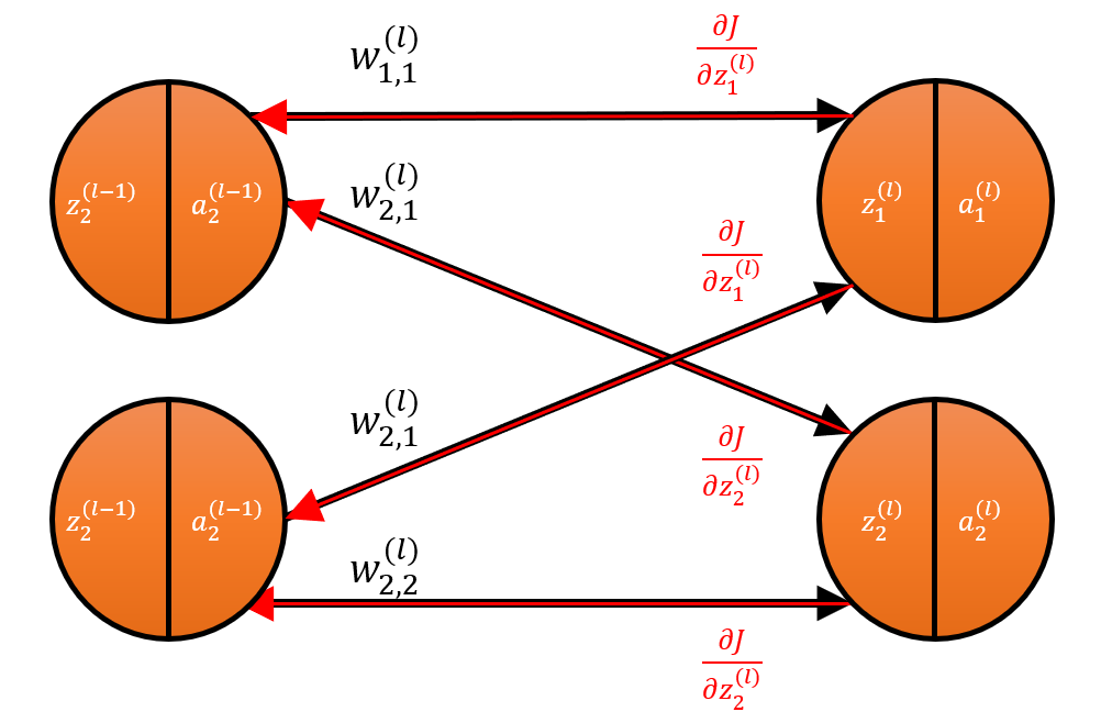
We know that each weight connects a particular node from a preceding layer to another in the current layer, and the same weight will be used on all the datapoints (examples) in the batch. Since each weight has a direct effect on only one particular node in the current layer, this also means that each weight only directly affects the batch of preactivations for the one particular node it impacts.
To properly illustrate this with the figure above, the weight \(w_{1,1}^{(l)}\) is a scalar, and it directly impacts the preactivation \({\vec{z}}_1^{(l)}\), which is a 1-by-\(m\) vector (i.e. the batch of preactivation values for node 1 in layer \(l\)). If you change only \(w_{1,1}^{(l)}\) and run a forward pass, then node 1 will be impacted (i.e. \({\vec{z}}_1^{(l)}\) will change too), but not node 2 (i.e. \({\vec{z}}_2^{(l)}\) will not change) or any other node.
Remember that, as shown in part 5, \({\vec{z}}_1^{(l)}\) is exactly row 1 of the matrix \(\mathbf{Z}^{(l)}\).
\[\mathbf{Z}^{(l)}=\left[\begin{matrix}{\vec{z}}_1^{(l)}\\{\vec{z}}_2^{(l)}\\\vdots\\{\vec{z}}_{n^{(l)}}^{(l)}\\\end{matrix}\right]=\left[\begin{matrix}z_{1,1}^{(l)}&z_{1,2}^{(l)}&\cdots&z_{1,m}^{(l)}\\z_{2,1}^{(l)}&z_{2,2}^{(l)}&\cdots&z_{2,m}^{(l)}\\\vdots&\vdots&\ddots&\vdots\\z_{n^{(l)},1}^{(l)}&z_{n^{(l)},2}^{(l)}&\cdots&z_{n^{(l)},m}^{(l)}\\\end{matrix}\right]\]In general, \({\vec{z}}_i^{(l)}\) is exactly row \(i\) of \(\mathbf{Z}^{(l)}\).
Therefore, it is more appropriate to expand \(\frac{\partial J}{\partial w_{1,1}^{(l)}}\) as follows:
\[\frac{\partial J}{\partial w_{1,1}^{(l)}}=\frac{\partial J}{\partial{\vec{z}}_1^{(l)}}\frac{\partial{\vec{z}}_1^{(l)}}{\partial w_{1,1}^{(l)}}\]We are making the derivative with respect to \(w_{1,1}^{(l)}\) expand into terms that we know are directly impacted by it. We also notice that the expansion is valid for matrix multiplication: \(\frac{\partial J}{\partial w_{1,1}^{(l)}}\) is a scalar, \(\frac{\partial J}{\partial{\vec{z}}_1^{(l)}}\) has a shape of 1-by-\(m\), and \(\frac{\partial{\vec{z}}_1^{(l)}}{\partial w_{1,1}^{(l)}}\) has a shape of \(m\)-by-1. Once again, when the procedure is logical, the math beautifully comes together.
Now let’s generalize the above chain rule expansion for any arbitrary scalar element of the cost gradient \(\frac{\partial J}{\partial\mathbf{W}^{(l)}}\):
\[\frac{\partial J}{\partial w_{i,h}^{(l)}}=\frac{\partial J}{\partial{\vec{z}}_i^{(l)}}\frac{\partial{\vec{z}}_i^{(l)}}{\partial w_{i,h}^{(l)}}\]There is more work involved in solving \(\frac{\partial J}{\partial{\vec{z}}_i^{(l)}}\), so let’s start with the low hanging fruit, \(\frac{\partial{\vec{z}}_i^{(l)}}{\partial w_{i,h}^{(l)}}\):
\[\frac{\partial{\vec{z}}_i^{(l)}}{\partial w_{i,h}^{(l)}}=\left[\begin{matrix}\frac{\partial z_{i,1}^{(l)}}{\partial w_{i,h}^{(l)}}\\\frac{\partial z_{i,2}^{(l)}}{\partial w_{i,h}^{(l)}}\\\vdots\\\frac{\partial z_{i,m}^{(l)}}{\partial w_{i,h}^{(l)}}\\\end{matrix}\right]\]Let \(\frac{\partial z_{i,j}^{(l)}}{\partial w_{i,h}^{(l)}}\) represent an arbitrary scalar element of the vector \(\frac{\partial{\vec{z}}_i^{(l)}}{\partial w_{i,h}^{(l)}}\). Then we solve \(\frac{\partial z_{i,j}^{(l)}}{\partial w_{i,h}^{(l)}}\):
\[\frac{\partial z_{i,j}^{(l)}}{\partial w_{i,h}^{(l)}}=\frac{\partial(\sum_{g=1}^{n^{(l-1)}}{w_{i,g}^{(l)}\cdot a_{i,j}^{(l-1)}})}{\partial w_{i,h}^{(l)}}=a_{h,j}^{(l-1)}\]Where the subscripts $ g $ and $ h $ both track the same quantity, which is the serial number of nodes in the layer preceding the current layer (i.e. layer $ l-1 $). That is, they both run from 1 to $ n^{(l-1)} $. The need for both subscripts is to allow for $ g $ and $ h $ not being equal, even though they both track the same quantity.
Therefore \(\frac{\partial{\vec{z}}_i^{(l)}}{\partial w_{i,h}^{(l)}}\) is:
\[\frac{\partial{\vec{z}}_i^{(l)}}{\partial w_{i,h}^{(l)}}=\left[\begin{matrix}a_{h,1}^{(l-1)}\\a_{h,2}^{(l-1)}\\\vdots\\a_{h,m}^{(l-1)}\\\end{matrix}\right]\]Based on what we saw in forward propagation, our activation matrix \(\mathbf{A}^{(l-1)}\) will be of the form:
\[\mathbf{A}^{(l-1)}=\left[\begin{matrix}{\vec{a}}_1^{(l-1)}\\{\vec{a}}_2^{(l-1)}\\\vdots\\a_{n^{(l)}}^{(l-1)}\\\end{matrix}\right]=\left[\begin{matrix}a_{1,1}^{(l-1)}&a_{1,2}^{(l-1)}&\cdots&a_{1,m}^{(l-1)}\\a_{2,1}^{(l-1)}&a_{2,2}^{(l-1)}&\cdots&a_{2,m}^{(l-1)}\\\vdots&\vdots&\ddots&\vdots\\a_{n^{(l)},1}^{(l-1)}&a_{n^{(l)},2}^{(l-1)}&\cdots&a_{n^{(l)},m}^{(l-1)}\\\end{matrix}\right]\]We observe that \(\frac{\partial{\vec{z}}_i^{(l)}}{\partial w_{i,h}^{(l)}}\) is simply the transpose of row \(h\) in \(\mathbf{A}^{(l-1)}\).
Therefore, the solution of \(\frac{\partial{\vec{z}}_i^{(l)}}{\partial w_{i,h}^{(l)}}\), in the form that we care for, is:
\[\frac{\partial{\vec{z}}_i^{(l)}}{\partial w_{i,h}^{(l)}}={\vec{a}}_h^{\left(l-1\right)T}\]We will return later to do more with the above.
So far, we can write \(\frac{\partial J}{\partial w_{i,h}^{(l)}}\) as:
\[\frac{\partial J}{\partial w_{i,h}^{(l)}}=\frac{\partial J}{\partial{\vec{z}}_i^{(l)}}{\vec{a}}_h^{\left(l-1\right)T}\]Similar to the procedure above, we look at \(\frac{\partial J}{\partial{\vec{z}}_i^{(l)}}\) elementwise:
\[\frac{\partial J}{\partial{\vec{z}}_i^{(l)}}=\left[\begin{matrix}\frac{\partial J}{\partial z_{i,1}^{(l)}}&\frac{\partial J}{\partial z_{i,2}^{(l)}}&\cdots&\frac{\partial J}{\partial z_{i,m}^{(l)}}\\\end{matrix}\right]\]Note that the cost gradient \(\frac{\partial J}{\partial\mathbf{Z}^{(l)}}\) looks like this:
\[\frac{\partial J}{\partial\mathbf{Z}^{(l)}}=\left[\begin{matrix}\frac{\partial J}{\partial z_{1,1}^{(l)}}&\frac{\partial J}{\partial z_{1,2}^{(l)}}&\cdots&\frac{\partial J}{\partial z_{1,m}^{(l)}}\\\frac{\partial J}{\partial z_{2,1}^{(l)}}&\frac{\partial J}{\partial z_{2,2}^{(l)}}&\cdots&\frac{\partial J}{\partial z_{2,m}^{(l)}}\\\vdots&\vdots&\ddots&\vdots\\\frac{\partial J}{\partial z_{n^{(l)},1}^{(l)}}&\frac{\partial J}{\partial z_{n^{(l)},2}^{(l)}}&\cdots&\frac{\partial J}{\partial z_{n^{(l)},m}^{(l)}}\\\end{matrix}\right]\]And therefore \(\frac{\partial J}{\partial{\vec{z}}_i^{(l)}}\) is simply row \(i\) in \(\frac{\partial J}{\partial\mathbf{Z}^{(l)}}\).
Let’s represent an arbitrary scalar element of the vector \(\frac{\partial J}{\partial{\vec{z}}_i^{(l)}}\) as \(\frac{\partial J}{\partial z_{i,j}^{(l)}}\), and solve for it. The chain rule expansion is:
\[\frac{\partial J}{\partial z_{i,j}^{(l)}}=\frac{\partial J}{\partial a_{i,j}^{(l)}}\frac{\partial a_{i,j}^{(l)}}{\partial z_{i,j}^{(l)}}\]All of the terms in the above equation are scalars. The logic for this chain rule expansion is that a given preactivation value for a node (and a specific datapoint), \(z_{i,j}^{(l)}\), directly influences the activation value of only that same node (and the same datapoint), i.e. \(a_{i,j}^{(l)}\).
There is more work involved in solving \(\frac{\partial J}{\partial a_{i,j}^{(l)}}\), so let’s start with the low hanging fruit, \(\frac{\partial a_{i,j}^{(l)}}{\partial z_{i,j}^{(l)}}\).
Based on the equation for forward propagation, we know that:
\[a_{i,j}^{(l)}=f(z_{i,j}^{\left(l\right)})\]Therefore, we can rewrite \(\frac{\partial a_{i,j}^{(l)}}{\partial z_{i,j}^{(l)}}\) as:
\[\frac{\partial a_{i,j}^{(l)}}{\partial z_{i,j}^{(l)}}=f'(z_{i,j}^{\left(l\right)})\]We will return later to do more with this.
Before we move on to \(\frac{\partial J}{\partial a_{i,j}^{(l)}}\), let’s pause and consider what we’ve done so far with solving the gradients for the hidden layers.
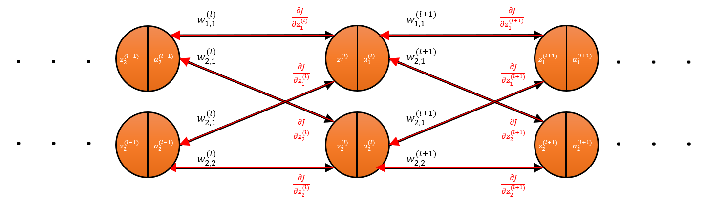
The image above that shows an arbitrary pathway in the hidden layers of the network and it actually captures exactly what we’ve done so far. Our quest started with an attempt to find \(\frac{\partial J}{\partial w_{i,h}^{(l)}}\), i.e. the rate of change of our cost \(J\) with respect to \(w_{i,h}^{(l)}\) (the weight for an arbitrary connection of a current layer \(l\)). To do that, we looked to \(z_{i,j}^{(l)}\). So, we expanded \(\frac{\partial J}{\partial w_{i,h}^{(l)}}\) in such a way that \(z_{i,j}^{(l)}\) appeared in the expansion, which led us to solve for the rate of change of our cost \(J\) with respect to \(z_{i,j}^{(l)}\). But we couldn’t completely solve it yet, so we looked to \(a_{i,j}^{(l)}\).
We expanded \(\frac{\partial J}{\partial z_{i,j}^{(l)}}\) in such a way that \(a_{i,j}^{(l)}\) appeared in the expansion. You see the pattern between our procedure thus far versus the arbitrary pathway presented in the image above? In order to get \(\frac{\partial J}{\partial w_{i,h}^{(l)}}\), we progressively stepped forward through the pathway. In fact, we were trying to work our way to the last layer, which we have already fully solved.
Notice that if we specify our arbitrary current layer \(l\) to be layer \(L-1\) (the layer before the last layer \(L\)), then the last layer L becomes the arbitrary layer \(l+1\). By the time we move on to layer \(L-2\) as the new current layer \(l\), layer \(L-1\) (which is now already fully solved) then becomes the new specification for the arbitrary layer \(l+1\). So, in fact, by getting our solution in terms of purely the arbitrary layer \(l+1\), we will complete the task of solving the entire network.
Therefore, following the pattern we’ve established, the next thing is to look to \(z_{p,j}^{(l+1)}\). We want to expand \(\frac{\partial J}{\partial a_{i,j}^{(l)}}\) in such a way that \(z_{p,j}^{(l+1)}\) appears somewhere in there. Now, how do we logically ensure that \(z_{p,j}^{(l+1)}\) appears in our chain rule expansion?
To answer that, we need to look at how a single scalar activation value from layer \(l\) influences the preactivations values of layer \(l+1\).
If you change \(a_{i,j}^{(l)}\), which means we’ve specified a particular datapoint as well (i.e. we are setting \(j\) to a fixed number), and run a forward pass on the network, then all the preactivations in the next layer, layer \(l+1\), will be impacted for that specified datapoint but not for any other datapoint.
To summarize, \(a_{i,j}^{(l)}\) directly impacts only column \(j\) in the matrix \(\mathbf{Z}^{(l+1)}\). Let’s represent column \(j\) of \(\mathbf{Z}^{(l+1)}\) as a column vector \({\vec{z}}_j^{(l+1)}\):
\[{\vec{z}}_j^{(l+1)}=\left[\begin{matrix}z_{1,j}^{(l+1)}\\z_{1,j}^{(l+1)}\\\vdots\\z_{n^{(l+1)},j}^{(l+1)}\\\end{matrix}\right]\]Therefore, we expand \(\frac{\partial J}{\partial a_{i,j}^{(l)}}\) as follows:
\[\frac{\partial J}{\partial a_{i,j}^{(l)}}=\frac{\partial{\vec{z}}_j^{(l+1)}}{\partial a_{i,j}^{(l)}}\frac{\partial J}{\partial{\vec{z}}_j^{(l+1)}}\]The reason we have \(\frac{\partial J}{\partial{\vec{z}}_j^{(l+1)}}\) at the end instead of next to the equality sign is to ensure matrix multiplication is valid, because \(\frac{\partial J}{\partial a_{i,j}^{(l)}}\) is a scalar, \(\frac{\partial{\vec{z}}_j^{(l+1)}}{\partial a_{i,j}^{(l)}}\) is a \(1\)-by-\(n^{(l)}\) vector and \(\frac{\partial J}{\partial{\vec{z}}_j^{(l+1)}}\) is an \(n^{(l)}\)-by-1 vector.
Also note that \(\frac{\partial J}{\partial{\vec{z}}_j^{(l+1)}}\) is also same as the \(j\)th column of \(\frac{\partial J}{\partial\mathbf{Z}^{(l+1)}}\):
\[\frac{\partial J}{\partial{\vec{z}}_j^{(l+1)}}=\left[\begin{matrix}\frac{\partial J}{\partial z_{1,1}^{(l+1)}}\\\frac{\partial J}{\partial z_{2,1}^{(l+1)}}\\\vdots\\\frac{\partial J}{\partial z_{n^{(l)},1}^{(l+1)}}\\\end{matrix}\right]\]Also notice that if we were trying to solve the gradients for the last hidden layer, i.e. \(l=\ L-1\), which is the layer before the output layer, then \(\frac{\partial J}{\partial\mathbf{Z}^{(l+1)}}\) will be \(\frac{\partial J}{\partial\mathbf{Z}^{(L)}}\), which we already computed.
In fact, by the time we are computing the gradients for any hidden layer \(l\), we will already have \(\frac{\partial J}{\partial\mathbf{Z}^{(l+1)}}\) (because we already computed it when computing gradients for \(l+1\)). This is the ultimate crux of backpropagation. This is what is meant by the “gradients flowing backward”, because you are directly using the gradients from a succeeding layer (layer \(l+1\)) to compute those of a preceding layer (layer \(l\)), and you continue that until you reach the input layer.
So, we have established that we don’t need to further solve for \(\frac{\partial J}{\partial{\vec{z}}_j^{(l+1)}}\) because we always already have it. Let’s tackle \(\frac{\partial{\vec{z}}_j^{(l+1)}}{\partial a_{i,j}^{(l)}}\):
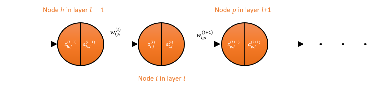
\[\frac{\partial{\vec{z}}_j^{(l+1)}}{\partial a_{i,j}^{(l)}}=\left[\begin{matrix}\frac{\partial z_{1,\ j}^{(l+1)}}{\partial a_{i,j}^{(l)}}&\frac{\partial z_{2,\ j}^{(l+1)}}{\partial a_{i,j}^{(l)}}&\cdots&\frac{\partial z_{n^{(l+1)},\ j}^{(l+1)}}{\partial a_{i,j}^{(l)}}\\\end{matrix}\right]\]So far, we’ve used the subscript \(i\) to track the serial number of nodes in current layer \(l\), and we have used \(g\) and \(h\) to track the serial number of nodes in layer \(l-1\). Now we formally introduce a new subscript \(p\) to track the serial number of nodes in layer \(l+1\) (we actually first mentioned it in the figure showing an arbitrary pathway through the network). Therefore, \(p\) counts from 1 to \(n^{(l+1)}\).
Let’s represent any arbitrary scalar element of the vector \(\frac{\partial{\vec{z}}_j^{(l+1)}}{\partial a_{i,j}^{(l)}}\) as \(\frac{\partial z_{p,\ j}^{(l+1)}}{\partial a_{i,j}^{(l)}}\). Let’s solve this arbitrary element.
\[\frac{\partial z_{p,j}^{(l+1)}}{\partial a_{i,j}^{(l)}}=\frac{\partial(\sum_{g=1}^{n^{\left(l\right)}}{w_{p,g}^{\left(l+1\right)}\cdot a_{g,j}^{\left(l\right)}})}{\partial a_{i,j}^{(l)}}=w_{p,i}^{\left(l+1\right)}\]Where $ w_{p,i}^{\left(l+1\right)} $ is the weight connecting node $ p $ in layer $ l+1 $ to node $ i $ in layer $ l $ as illustrated in the figure above showing an arbitrary pathway through the network.
Therefore, we have:
\[\frac{\partial{\vec{z}}_j^{(l+1)}}{\partial a_{i,j}^{(l)}}=\left[\begin{matrix}\frac{\partial z_{1,\ j}^{(l+1)}}{\partial a_{i,j}^{(l)}}&\frac{\partial z_{2,\ j}^{(l+1)}}{\partial a_{i,j}^{(l)}}&\cdots&\frac{\partial z_{n^{(l+1)},\ j}^{(l+1)}}{\partial a_{i,j}^{(l)}}\\\end{matrix}\right]=\left[\begin{matrix}w_{1,i}^{\left(l+1\right)}&w_{2,i}^{\left(l+1\right)}&\cdots&w_{n^{(l+1)},i}^{\left(l+1\right)}\\\end{matrix}\right]\]Similar to the other solutions we’ve seen, we notice that the solution to \(\frac{\partial{\vec{z}}_j^{(l+1)}}{\partial a_{i,j}^{(l)}}\) is simply column \(i\) of the matrix \(\mathbf{W}^{(l+1)}\) transposed.
Therefore \(\frac{\partial J}{\partial a_{i,j}^{(l)}}\) is:
\[\frac{\partial J}{\partial a_{i,j}^{(l)}}=\frac{\partial{\vec{z}}_j^{(l+1)}}{\partial a_{i,j}^{(l)}}\frac{\partial J}{\partial{\vec{z}}_j^{(l+1)}}=\left[\begin{matrix}w_{1,i}^{\left(l+1\right)}&w_{2,i}^{\left(l+1\right)}&\cdots&w_{n^{(l+1)},i}^{\left(l+1\right)}\\\end{matrix}\right]\left[\begin{matrix}\frac{\partial J}{\partial z_{1,1}^{(l+1)}}\\\frac{\partial J}{\partial z_{2,1}^{(l+1)}}\\\vdots\\\frac{\partial J}{\partial z_{n^{(l)},1}^{(l+1)}}\\\end{matrix}\right]\]We always already have \(\mathbf{W}^{(l+1)}\) (either the originally initialized matrix or the one that has been updated during a previous backward pass), and as pointed out earlier, we also have matrix \(\frac{\partial J}{\partial Z^{(l+1)}}\) (and we mentioned earlier that \(\frac{\partial J}{\partial{\vec{z}}_j^{(l+1)}}\) is simply the \(j\)th column of it). Therefore, there is nothing left to solve. We now have \(\frac{\partial J}{\partial a_{i,j}^{(l)}}\) fully characterized. Working backward, we also notice that we now also have \(\frac{\partial J}{\partial z_{i,j}^{(l)}}\) and \(\frac{\partial J}{\partial w_{i,h}^{(l)}}\) all fully characterized as well.
We’ve therefore solved the network and completed our execution of backpropagation symbolically. What remains is to now compact everything back into beautiful tensors.
Compacting the gradients of the hidden layers
Our ultimate goal is to solve the Jacobians \(\frac{\partial J}{\partial\mathbf{W}^{(l)}}\) and \(\frac{\partial J}{\partial\mathbf{B}^{(l)}}\) so that we can update the parameters (weights and biases) via gradient descent.
As we already mentioned, \(a_{i,j}^{(l)}\) is the activation for an arbitrary node \(i\) in layer \(l\) for example \(j\). Essentially, \(a_{i,j}^{(l)}\) is simply an arbitrary scalar element of the matrix \(\mathbf{A}^{(l)}\). Therefore, similarly, \(\frac{\partial J}{\partial a_{i,j}^{(l)}}\) is an arbitrary scalar element of the matrix \(\frac{\partial J}{\partial\mathbf{A}^{(l)}}\):
\[\frac{\partial J}{\partial\mathbf{A}^{(l)}}=\left[\begin{matrix}\frac{\partial J}{\partial a_{1,1}^{(l)}}&\frac{\partial J}{\partial a_{1,2}^{(l)}}&\cdots&\frac{\partial J}{\partial a_{1,m}^{(l)}}\\\frac{\partial J}{\partial a_{2,1}^{(l)}}&\frac{\partial J}{\partial a_{2,2}^{(l)}}&\cdots&\frac{\partial J}{\partial a_{2,m}^{(l)}}\\\vdots&\vdots&\ddots&\vdots\\\frac{\partial J}{\partial a_{n^{(l)},1}^{(l)}}&\frac{\partial J}{\partial a_{n^{(l)},2}^{(l)}}&\cdots&\frac{\partial J}{\partial a_{n^{(l)},m}^{(l)}}\\\end{matrix}\right]\]From the solution of \(\frac{\partial J}{\partial a_{i,j}^{(l)}}\), we know that each scalar element of \(\frac{\partial J}{\partial\mathbf{A}^{(l)}}\) is computed from the multiplication of the \(i\)th column of \(\mathbf{W}^{(l+1)}\) transposed (i.e. \(\mathbf{W}^{(l+1)T}\)) and the \(j\)th column of \(\frac{\partial J}{\partial\mathbf{Z}^{(l+1)}}\).
In other words:
\[\frac{\partial J}{\partial\mathbf{A}^{\left(l\right)}}=\left[\begin{matrix}w_{1,1}^{\left(l+1\right)}&w_{1,2}^{\left(l+1\right)}&\cdots&w_{1,n^{\left(l\right)}}^{\left(l+1\right)}\\w_{2,1}^{\left(l+1\right)}&w_{2,2}^{\left(l+1\right)}&\cdots&z_{2,n^{\left(l\right)}}^{\left(l+1\right)}\\\vdots&\vdots&\ddots&\vdots\\w_{n^{\left(l+1\right)},1}^{\left(l+1\right)}&w_{n^{\left(l+1\right)},2}^{\left(l\right)}&\cdots&w_{n^{\left(l+1\right)},n^{\left(l\right)}}^{\left(l+1\right)}\\\end{matrix}\right]^T\left[\begin{matrix}\frac{\partial J}{\partial z_{1,1}^{\left(l+1\right)}}&\frac{\partial J}{\partial z_{1,2}^{\left(l+1\right)}}&\cdots&\frac{\partial J}{\partial z_{1,m}^{\left(l+1\right)}}\\\frac{\partial J}{\partial z_{2,1}^{\left(l+1\right)}}&\frac{\partial J}{\partial z_{2,2}^{\left(l+1\right)}}&\cdots&\frac{\partial J}{\partial z_{2,m}^{\left(l+1\right)}}\\\vdots&\vdots&\ddots&\vdots\\\frac{\partial J}{\partial z_{n^{\left(l+1\right)},1}^{\left(l+1\right)}}&\frac{\partial J}{\partial z_{n^{\left(l+1\right)},2}^{\left(l+1\right)}}&\cdots&\frac{\partial J}{\partial z_{n^{\left(l+1\right)},m}^{\left(l+1\right)}}\\\end{matrix}\right]\]And the above condenses to:
\[\frac{\partial J}{\partial\mathbf{A}^{\left(l\right)}}=\mathbf{W}^{(l+1)T}\frac{\partial J}{\partial\mathbf{Z}^{(l+1)}}\]Also note that the above equation can also be rewritten in this form (which is my preferred version, and it’s the version I implemented in code in part 7):
\[\frac{\partial J}{\partial\mathbf{A}^{\left(l-1\right)}}=\mathbf{W}^{(l)T}\frac{\partial J}{\partial\mathbf{Z}^{(l)}}\]Moving on to \(\frac{\partial J}{\partial z_{i,j}^{(l)}}\), we established earlier that:
\[\frac{\partial J}{\partial z_{i,j}^{(l)}}=\frac{\partial J}{\partial a_{i,j}^{(l)}}\frac{\partial a_{i,j}^{(l)}}{\partial z_{i,j}^{(l)}}=\frac{\partial J}{\partial a_{i,j}^{(l)}}f'(z_{i,j}^{\left(l\right)})\]We know \(\frac{\partial J}{\partial z_{i,j}^{(l)}}\), \(\frac{\partial J}{\partial a_{i,j}^{(l)}}\), and \(z_{i,j}^{\left(l\right)}\) represent the arbitrary scalar elements of \(\frac{\partial J}{\partial\mathbf{A}^{\left(l\right)}}\), \(\frac{\partial J}{\partial\mathbf{Z}^{\left(l\right)}}\) and \(\mathbf{Z}^{(l)}\). This also means that \(f'(z_{i,j}^{\left(l\right)})\) is simply the arbitrary scalar element of \(f'(Z^{\left(l\right)})\), which is simply the elementwise application of the function \(f'\) on the matrix \(\mathbf{Z}^{\left(l\right)}\), where \(f\) is an activation function and \(f’\) is its derivative. With this, we discover that \(\frac{\partial J}{\partial\mathbf{Z}^{\left(l\right)}}\) is simply the elementwise multiplication of \(\frac{\partial J}{\partial\mathbf{A}^{\left(l\right)}}\) and \(f'(\mathbf{Z}^{\left(l\right)})\):
\[\frac{\partial J}{\partial\mathbf{Z}^{\left(l\right)}}=\frac{\partial J}{\partial\mathbf{A}^{\left(l\right)}}\odot f'(\mathbf{Z}^{\left(l\right)})\]Finally, we tackle \(\frac{\partial J}{\partial w_{i,h}^{(l)}}\), which is the arbitrary scalar element of \(\frac{\partial J}{\partial\mathbf{W}^{(l)}}\).
We already solve it this far:
\[\frac{\partial J}{\partial w_{i,h}^{(l)}}=\frac{\partial J}{\partial{\vec{z}}_i^{(l)}}{\vec{a}}_h^{\left(l-1\right)T}\]And we already noted that \(\frac{\partial J}{\partial{\vec{z}}_i^{(l)}}\) is exactly row \(i\) in \(\frac{\partial J}{\partial Z^{(l)}}\) and \({\vec{a}}_h^{\left(l-1\right)T}\) is exactly the transpose of row \(h\) in \(\mathbf{A}^{(l-1)}\). We’ve just described matrix multiplication between \(\frac{\partial J}{\partial\mathbf{Z}^{(l)}}\) and \(\mathbf{A}^{(l-1)T}\).
Therefore:
\[\frac{\partial J}{\partial\mathbf{W}^{(l)}}=\frac{\partial J}{\partial\mathbf{Z}^{(l)}}\mathbf{A}^{(l-1)T} = \frac{\partial J}{\partial\mathbf{A}^{\left(l\right)}}\odot f'(\mathbf{Z}^{\left(l\right)})\mathbf{A}^{(l-1)T}\]The last gradient we need to solve is \(\frac{\partial J}{\partial\mathbf{B}^{(l)}}\). I will leave that to the reader (as the procedure is vastly simpler than what we’ve done so far). The final result is:
\[\frac{\partial J}{\partial\mathbf{B}^{(l)}}=\sum_{j=1}^{m}\left(\frac{\partial J}{\partial\mathbf{Z}^{(l)}}\right)_j\]We have now fully solved our network symbolically and have all our gradients as compact matrices. But you may have noticed that the results for the hidden layers are identical to the results for the output layer, except for \(\frac{\partial J}{\partial A^{\left(l\right)}}\) (for \(l<L\), i.e. hidden layers) and \(\frac{\partial J}{\partial A^{\left(L\right)}}\), which do not have identical results.
This is completely logical as there is no layer beyond the output layer \(L\), instead the next set of computations after the output layer is the calculation of the cost (in a sense, the cost is the final component in any arbitrary pathway in the network). Hence \(\frac{\partial J}{\partial\mathbf{A}^{\left(L\right)}}\) is directly the derivative of the cost function, while in the case of \(\frac{\partial J}{\partial\mathbf{A}^{(l)}}\) for \(l<L\), we look to the next component in our arbitrary pathway (which is the next layer of nodes, layer \(l+1\)) for answers.
Updating parameters via gradient descent
The next stage of backward pass is to update our parameters. There are many updating schemes out there, but I will show gradient descent. It is one of the oldest (was proposed by the mathematician Augustin-Louis Cauchy in 1847) and still widely in use today. The procedure is exactly the same as what we saw with an artificial neuron in part 3.
\[w_{new}=w_{old}-\gamma\frac{\partial J}{\partial w_{old}}\] \[b_{new}=b_{old}-\gamma\frac{\partial J}{\partial b_{old}}\]The equations are applied to each of the parameter values in the network. That is, these equations are applied to each scalar element of the matrices \(\mathbf{W}\) and \(\mathbf{B}\).
All that’s left now is to implement in code the equations presented in this article.
comments powered by Disqus