Catching AI with its pants down: Understand an Artificial Neuron from Scratch
| We will strip the mighty, massively hyped, highly dignified AI of its cloths, and bring its innermost details down to earth! |
- Prologue
- The brain as a function
- Toy dataset for this blog series
- Artificial neuron
- Activation functions
- Loss function
Prologue
This is part 2 of this blog series, Catching AI with its pants down. This blog series aims to explore the inner workings of neural networks and show how to build a standard feedforward neural network from scratch.
In this part, I will go over the biological inspiration for the artificial neuron and its mathematical underpinnings.
| Parts | The complete index for Catching AI with its pants down |
|---|---|
| Pant 1 | Some Musings About AI |
| Pant 2 | Understand an Artificial Neuron from Scratch |
| Pant 3 | Optimize an Artificial Neuron from Scratch |
| Pant 4 | Implement an Artificial Neuron from Scratch |
| Pant 5 | Understand a Neural Network from Scratch |
| Pant 6 | Optimize a Neural Network from Scratch |
| Pant 7 | Implement a Neural Network from Scratch |
| Pant 8 | Demonstration of the Models in Action |
Notation for tensors
Just like in every article for this blog series, unless explicitly started otherwise, matrices (and higher-order tensors, which should be rare in this blog series) are denoted with boldfaced, non-italic, uppercase letters; vectors are denoted with non-boldfaced, italic letters accented with a right arrow; and scalars are denoted with non-boldfaced, italic letters. E.g. \(\mathbf{A}\) is a matrix, \(\vec{a}\) is a vector, and \(a\) or \(A\) is a scalar.
The brain as a function
The computational theory of mind (CTM) says that we can interpret human cognitive processes as computational functions. That is, the human mind behaves just like a computer.
Note that while CTM is considered a decent model for human cognition (it was the unchallenged standard in the 1960s and 1970s and still widely subscribed to), no one has been able to show how consciousness can emerge from a system modelled on the basis of this theory, but that’s another topic for another time.
For a short primer on CTM, see this article from the Stanford Encyclopedia of Philosophy.
According to CTM, if we have a mathematical model of all the computations that goes on in the brain, we should, one day, be able to replicate the capabilities of the brain with computers. But how does the brain do what it does?
Biological neuron
In a nutshell, the brain is made up of two main kinds of cells: glial cells and neurons (a.k.a. nerve cells). There are about 86 billion neurons and even more glial cells in the nervous system (brain, spinal cord and nerves) of an adult human. The primary function of glial cells is to provide physical protection and other kinds of support to neurons, so we are not very interested in glial cells here. It’s the neuron we came for.
The primary function of biological neurons is to process and transmit signals, and there are three main types: sensory neurons (concentrated in your sensory organs like eyes, ears, skin, etc.), motor neurons (carry signals between the brain and spinal cord, and from both to the muscles), and interneurons (found only in the brain and spinal cord, and they process information).
For instance, when you grab a very hot cup, sensory neurons in the nerves of your fingers send a signal to interneurons in your spinal cord. Some interneurons pass the signal on to motor neurons in your hand, which causes you to drop the cup, while other interneurons send a signal to those in your brain, and you experience pain.
So clearly, in order to start modelling the brain, we have to first understand the neuron and try to model it mathematically.
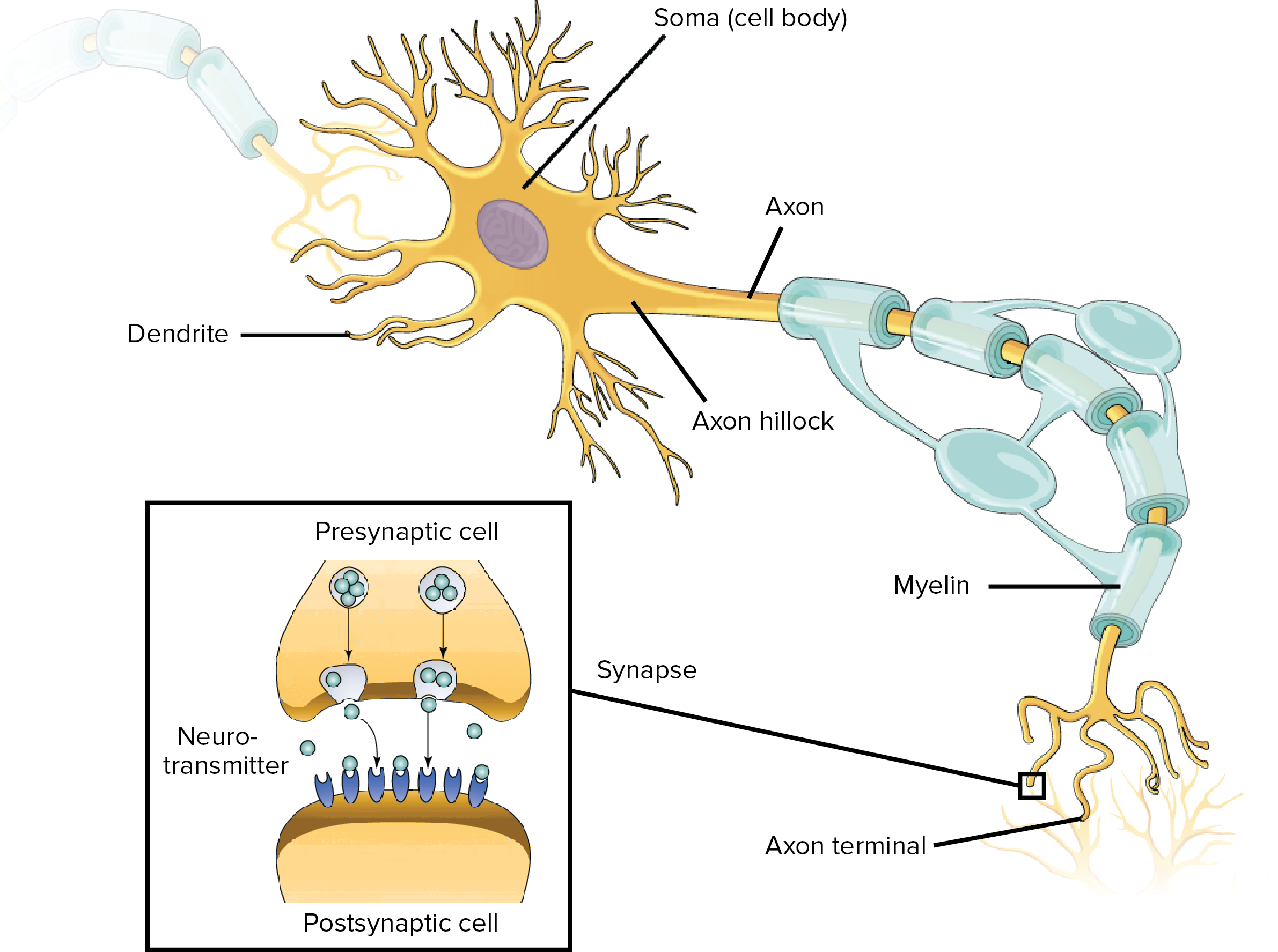
Neurons in the brain usually work in groups known as neural circuits (or biological neural networks), where they provide some biological function. A neuron has 3 main parts: the dendrites, soma (cell body) and axon.
The dendrite of one neuron is connected to the axon terminal of another neuron, and so on, resulting in a network of connected neurons. The connection between two neurons is known as the synapse, and there is no actual physical contact, as the neurons don’t actually touch each other.
Instead, a neuron will release chemicals (neurotransmitters) that carry the electrical signal to the dendrite of the next neuron. The strength of the transmission is known as the synaptic strength. The more often signals are transmitted across a synapse, the stronger the synaptic strength becomes. This rule, commonly known as Hebb’s rule (introduced in 1949 by Donald Hebb), is colloquially stated as, “neurons that fire together wire together.”
Neurons receive signal via their dendrites and outputs signal via their axon terminals. And each neuron can be connected to thousands of other neurons. When a neuron receives signals from other neurons, it combines all the input signals and generates a voltage (known as graded potential) on the membrane of the soma that is proportional, in size and duration, to the sum of the input signals.
The graded potential gets smaller as it travels through the soma to reach the axon. If the graded potential that reaches the trigger zone (near the axon hillock) is higher than a threshold value unique to the neuron, the neuron fires a huge electric signal, called the action potential, that travels down the axon and through the synapse to become the input signal for the neurons downstream.
Toy dataset for this blog series
Before we advance any further to artificial neurons, let’s introduce a toy dataset that will accompany subsequent discussions and be used to provide vivid illustration.
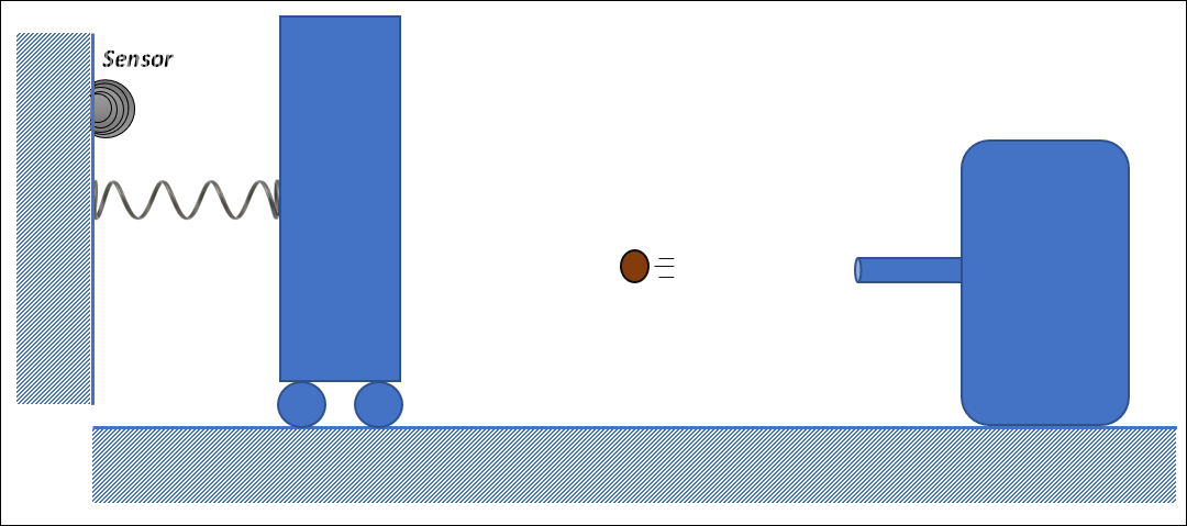
You can think of the data as being generated from an experiment where a device launches balls of various masses unto a board that can roll backward, and when it does roll back all the way to touch the sensor, that shot is recorded as high energy, otherwise it is classified as low energy.
Below is an excerpt of the dataset:
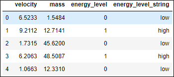
The dataset has two features or inputs, i.e. velocity and mass, and a single output, which is energy level and it is binary. The last two columns are exactly the same, just that the third is the numerical version of the last and is what we actually use because we need to crunch numbers. In classification, the labels are converted to numbers for the learning process. The dataset was simulated using classical mechanics and random uniform noise.
The full toy dataset can be found here.
Artificial neuron
In the 1950s, the psychologist Frank Rosenblatt introduced a very simple mathematical abstraction of the biological neuron. He developed a model that mimicked the following behavior: signals that are received from dendrites are sent down the axon once the strength of the input signal crosses a certain threshold. The outputted signal can then serve as an input to another neuron. Rosenblatt named this mathematical model the perceptron.
Rosenblatt’s original perceptron was a simple Heaviside function that outputs zero if the input signal is equal to or less than 0, and outputs 1 if the input is greater than zero. Therefore, zero was the threshold above which an input makes the neuron to fire. The original perceptron is an example of an artificial neuron, and we will see other examples.
An artificial neuron is simply a mathematical function that serves as the elementary unit of a neural network. It is also known as a node or a unit, with the latter name being very common in machine learning publications. I may jump between these names, and it’s not bad if you get used to that, as all of these names are common.
Mathematical representation
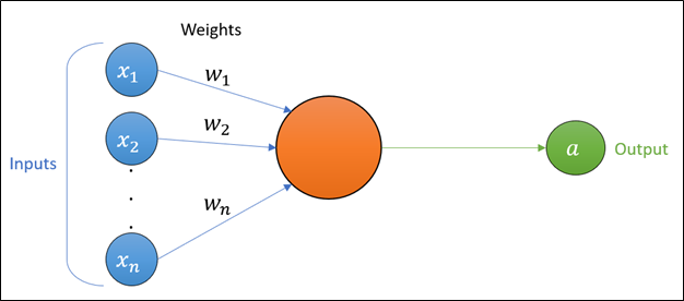
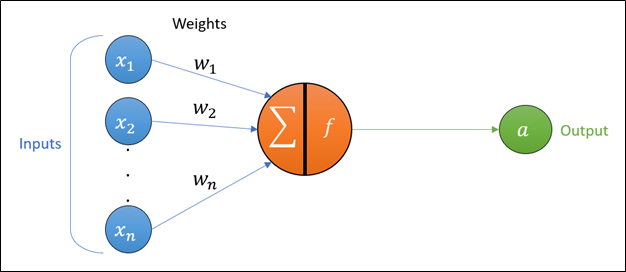
This mathematical function has a collection of inputs, \(x_1,x_2,\ \ldots,\ x_n\), and a single output, \(a\), commonly known as the activation value (or post-activation value), or often without the term “value” (i.e. simply activation).
But what then happens inside a unit (an artificial neuron)?
The inputs that are fed into a unit are used in two key operations in order to generate the activation:
-
Summation: The inputs ($ x_i $) are multiplied with the weights (\(w_i\)), and the products are summed together. This summation is sometimes called the preactivation value, or without the term “value”.
-
Activation function (a.k.a. transfer function): the resulting sum (i.e. the preactivation) is passed through a mathematical function.
The activation value can be thought of as a loose adaptation of the biological action potential, and the weights imitate synaptic strength.
The inputs to the neuron, \(x_i\), can themselves be activation values from other neurons. However, at this stage, where we are focusing on the model for only one artificial neuron, we will set the inputs to be the data, which loosely represents the stimuli received by the sensory organs in the biological analogy.
The algebraic representation of an artificial neuron is:
\[a=f\left(z\right)\]Where $ a $ is the activation, $ z $ is the preactivation, and $ f $ is the activation function (in the case of the original perceptron, this is the Heaviside function).
The preactivation $ z $ is computed as:
\[z=w_1\ \cdot x_1+w_2\ \cdot x_2+\ldots+w_n\ \cdot x_n+w_0=\sum_{i=0}^{n}{w_i\ \cdot x_i}\]Where $ n $ is the number of features in our dataset, which means $ i $ tracks the features (i.e. it is the serial number of the features).
Now check back with the diagram of an artificial neuron and see if you can make the connection between the equations and the diagram. Don’t move on unless you already have this down.
Math with some numbers
It’s important to start putting these equations in the context of data. Using our toy dataset (introduced above), the application of this equation can be demonstrated by taking any datapoint and subbing the values into the above equation. For instance, if we sub in the 0th datapoint (6.5233, 1.5484, 0), we get:
\[z=w_1\ \cdot 6.5233+w_2\ \cdot1.5484+w_0\]We will keep the weights as variables for now because we don’t know the appropriate weights for this dataset (that’s a problem we leave for when we train the artificial neuron). The complete algebraic representation of the original perceptron, which has the Heaviside function as its activation function, is:
\[a = \begin{cases} 1 &\text{if } z > 0 \\ 0 &\text{if } z \leq 0 \end{cases}\]If you took a moment to really look at the equation for preactivation, you will notice something is off, compared to the artificial neuron diagram. Where did \(w_0\) come from? And what about \(x_0\)? The answer is the “bias term”. That’s the name for \(w_0 \cdot x_0\). It allows our function to shift, and its presence is purely a mathematical necessity.
The variable \(w_0\) is known as the bias, and \(x_0\) (commonly referred to as the bias node) is a constant that is always equal to one and has nothing to do with the data, unlike \(x_1\) to \(x_n\) that comes from the data (e.g. the pixels of the images in the case of an image classification task). That’s how \(w_0 \cdot x_0\) reduces to just \(w_0\).
Moreover, we will henceforth refer to \(w_0\) as \(b\), and this is the letter often used in literature to represent the bias. The weights (\(w_1,\ w_2,\ \ldots,\ w_n\)) and bias (\(w_0\) or \(b\)) collectively are known as the parameters of the artificial neuron.
The need for the bias term:
As already mentioned, the bias term allows our function to shift. Its presence is purely a mathematical necessity.
Where $ w_1 $ is the slope of the line, and $ w_0 $ is the vertical axis intercept. But what if we omitted the vertical axis intercept? Well, we may never be able to perfectly fit a line through those two datapoints. Actually, we will never be able to perfectly fit a straight line through both points if it happens that the line that perfectly fits on them does not go through the origin (which is intercept of zero). 
In general, it goes like this: If we have a function $ f(x) $, then $ f\left(x\right)+c $ applies a vertical shift of $ c $ on the function. Whereas, $ f(x+c) $ applies a horizontal shift of $ c $. This should be enough refresher of this high school topic, and it is also the reason why we need the bias term. But the presence of the bias term in our artificial neuron equation means that the true diagram should look like this: 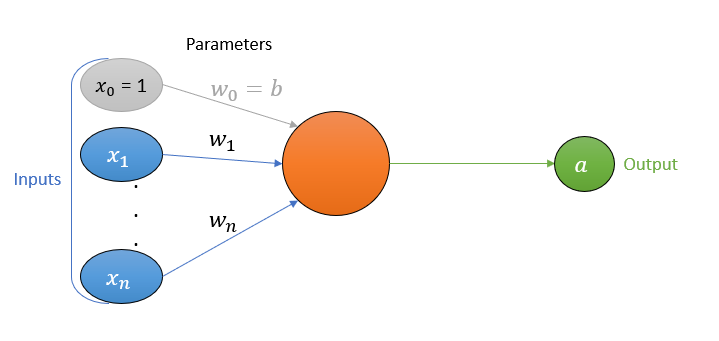
|
We observe that the equation for an artificial neuron can be condensed into this:
\[a=f(x;w,b)\]Where $ x=(x_1,\ x_2,\ldots,\ x_n) $ and $ w=(w_1,\ w_2,\ldots,w_n) $
The equation is read as $ a $ is a function of $ x $ parameterized by $ w $ and $ b $. And in fact, we’ve just introduced vectors. One geometrical interpretation of a vector in a given space (could be 2D, 3D space, etc.) is that it is a point with a “sense” of direction, or just an arrow pointing from the origin to a point.
So effectively we have this:
\[a=f(\vec{x};\vec{w},b)\]Where $ \vec{x}=\left[\begin{matrix}x_1\\x_2\\\vdots\\x_n\\\end{matrix}\right] $ and $ \vec{w}=\left[\begin{matrix}w_1\\w_2\\\vdots\\w_n\\\end{matrix}\right]^T $.
If you are doubting, then check if this equation is correct (spoiler alert: it is correct!):
\[\vec{w}\ \cdot\vec{x}=\vec{w}\vec{x}=\sum_{i=1}^{n}{w_i\ \cdot x_i}\]Note that the lack of any symbols between $ \vec{w} $ and $ \vec{x} $ signifies vector-vector multiplication, which is same as dot product of vectors. It's also common for vector-matrix multiplication and matrix-matrix multiplication to be presented the same way, because they are all kinds of matrix multiplication. The dot symbol ($ \cdot $) between any two scalars means regular multiplication of scalars, and it means dot product for vectors.
A useful idea for converting an equation or a system of them into a matrix or vector equation is to recognize that:
- Vector-vector multiplication is same as the dot product of two vectors.
- Dot product is simply elementwise multiplication followed by summation of the products.
- Vector-matrix multiplication directly reduces to the dot product between the row or column vectors of a matrix and a vector. This makes vector-matrix multiplication, which is a subset of matrix multiplication, one example of tensor contraction. (We will revisit this later).
So, when you see a pair of scalars getting multiplied and then the products from all such pairs are added (the formal name for this is linear combination), you should immediately suspect that such an equation may be easily substituted with a “tensorized” version.
What is a tensor?
You probably already think of a vector as an array with one dimension (or axis). This makes it a first-order tensor, and a matrix is a second-order tensor as it has two axes. Similar objects with more than two axes are higher order tensors.
|
The equations we’ve seen above are under the premise that we will be handling only one datapoint at a time. But we need to be able to handle more than one datapoint simultanously (we also need this when we start looking into neural networks because operations on matrices are easily parallelized). For this reason, we will do one more important thing to the equations we’ve seen above, which is to take them to matrix form.
Improvement in parallelized computing is a huge reason deep learning returned to the spotlight in the last decade. Parallelization is also the reason GPUs have become a champion for machine learning, because they have thousands of cores unlike CPUs which typically have cores that number in the single digits.
Going back to our toy dataset, if we wanted to compute preactivations for the first three datapoints at once, we get these three equations (and please always keep in mind that \(w_0=b\)):
\[z=w_1\ \cdot6.5233+w_2\ \cdot1.5484+w_0\] \[z=w_1\ \cdot9.2112+w_2\ \cdot12.7141+w_0\] \[z=w_1\ \cdot1.7315+w_2\ \cdot45.6200+w_0\]Clearly, we need a new subscript to keep track of multiple datapoints, because it’s misleading to keep equating every datapoint to just \(z\). So, we do something like this:
\[z_j=w_1\ \cdot x_{1,j}+w_2\ \cdot x_{2,j}+\ldots+w_n\ \cdot x_{n,j}+w_0=\sum_{i=1}^{n}{w_i\ \cdot x_{i,j}+b}\]Where the subscript $ j $ is the serial number that keeps track of datapoints. Or you can think of it as, $ i $ tracks the columns and $ j $ tracks rows in our toy dataset. Note that $ w_0 $ is same as $ b $.
So now we can write them as:
\[z_1=w_1\ \cdot6.5233+w_2\ \cdot1.5484+b\] \[z_2=w_1\ \cdot9.2112+w_2\ \cdot12.7141+b\] \[z_3=w_1\ \cdot1.7315+w_2\ \cdot45.6200+b\]Note that the numerical subscript on \(z\) above is not counterpart to that on \(w\). The former tracks datapoints (rows in our toy dataset), and the latter tracks features (columns in our toy dataset). It’s all much clearer when they are all purely in algebra form.
You can already notice the system of equations. And if it had been a batch of 100 datapoints, or even the entire dataset, it starts becoming unwieldy to carry around thousands of equations. Therefore we vectorize!
We summarize the preactivations for all the datapoints in our batch:
\[\vec{z}=all\ z_j\ in\ the\ batch=[\begin{matrix}z_1&z_2&\cdots&z_m\\\end{matrix}]\]Where $ m $ is the number of datapoints in our batch.
What’s “the batch” all about? In deep learning, it’s very common to deal with very large datasets that may be too big or inefficient to load into memory all at once. So typically we sample out a portion of our dataset, which we call a batch, and use it to train our model. That’s one iteration of training. We repeat the sampling for the second iteration, and continue for as many iterations as we choose to.
Now we have all the ingredients to convert to matrix format. Our system of equation, will go from this:
\[z_1=w_1\ \cdot x_{1,1}+w_2\ \cdot x_{2,1}+\ldots+w_n\ \cdot x_{n,1}+w_0\] \[z_2=w_1\ \cdot x_{1,2}+w_2\ \cdot x_{2,2}+\ldots+w_n\ \cdot x_{n,2}+w_0\] \[\vdots\] \[z_m=w_1\ \cdot x_{1,m}+w_2\ \cdot x_{2,m}+\ldots+w_n\ \cdot x_{n,m}+w_0\]To this matrix equation:
\[\vec{z}\ =\ \vec{w}\mathbf{X}\ + \vec{b}\]Note that the lack of any symbols between $ \vec{w} $ and $ \mathbf{X} $ signifies matrix-vector multiplication, i.e. matrix multiplication between vector and matrix.
I encourage you to rework the matrix equation back into the flat form if you’re unclear on how the two are the same. I promise, it will be a great refresher of math you probably saw in high school or first year of university.
The variable \(\vec{z}\) is a \(1\)-by-\(m\) vector, and if only one datapoint, will be a vector of only one entry (which is equivalent to a scalar).
The parameter \(\vec{w}\) is always going to be a \(1\)-by-\(n\) vector, regardless of the number of datapoints. Its size depends on the number of features \(n\).
\[\vec{w}=\left[\begin{matrix}w_1\\w_2\\\vdots\\w_n\\\end{matrix}\right]^T\]The variable \(b\) is a \(1\)-by-\(m\) vector. Fundamentally, however, the bias is a scalar (or a \(1\)-by-\(1\) vector) regardless of the number datapoints in the batch.
There is only one bias for a neuron, and it’s simply the weight for the bias node, just like each of the other weights. It only gets stretched into a \(1\)-by-\(m\) vector to match the shape of \(z\), so that the matrix equation is valid. The stretching involves repeating the elements to fill up the stretched-out vector. When coding in Python and using the NumPy library for your computations, it’s good to know that this stretching (also called broadcasting) is already baked into the library.
Therefore the full answer for the shape of \(b\) is that it is fundamentally a scalar (or a $ 1 $-by-$ 1 $ vector) that gets broadcasted into a vector of the right shape during the computation involved in the matrix equation for computing the preactivation. (If this still doesn’t make sense here, return to it later after you finish part 4).
We must keep in mind that \(b\) is a parameter of the estimator, and it would be very counterproductive to define it in a way that binds it to the number of examples (datapoints) in a batch. This is why its fundamental form is a scalar.
Here are some problems we would have if we defined \(b\) to be fundamentally a \(1\)-by-\(m\) vector:
-
The neuron becomes restricted to a fixed batch size. That is, the batch size we use to train the neuron becomes a fixture of the neuron, to the point that we can’t use the neuron to carry out predictions or estimations for a different batch size.
-
Each example in the batch will have a different corresponding value for $ b $. This is not even the case for $ w $, and it is just simply improper for the parameters to change from datapoint to datapoint. If that happened, then it means the model is not identical for all datapoints. Absolutely appalling.
When \(b\) is broadcasted into the \(1\)-by-\(m\) vector \(\vec{b}\), it is simply the scalar value \(b\) repeating \(m\) times. It looks like this:
\[\vec{b}=\left[\begin{matrix}b&b&\cdots&b\\\end{matrix}\right]\]The intuition is that you are applying the same bias to all the datapoint in any given batch, the same way you are applying the same group of weights to all the datapoint.
Because the bias is fundamentally a scalar, it is normal to write the equation as:
\[\vec{z}\ =\vec{w}\mathbf{X}\ +b\]The variables \(\mathbf{X}\) will depend on the shape of the input data that gets fed to the neuron. It could be a vector or matrix (and in neural networks they could even be higher order tensors). When dealing with multiple datapoints, it’s an \(n\)-by-\(m\) matrix, and when a single datapoint it’s an \(n\)-by-\(1\) vector. It looks like this:
\[\mathbf{X}=\left[\begin{matrix}x_{1,1}&x_{1,2}&\cdots&x_{1,m}\\x_{2,1}&x_{2,2}&\cdots&x_{2,m}\\\vdots&\vdots&\ddots&\vdots\\x_{n,1}&x_{n,2}&\cdots&x_{n,m}\\\end{matrix}\right]\]Keep in mind that these statements about the shapes of these tensors are all for a single artificial neuron, as there are some changes when moving unto neural networks (a network of neurons).
Let’s illustrate with our toy dataset how the preactivation equation works in matrix format. Let’s say we decide that our batch size will be 3, which means we will feed our neuron 3 datapoints (3 rows from our toy dataset), then our \(\mathbf{X}\) will look like this:
\[\mathbf{X}=\left[\begin{matrix}6.5233&9.2112&1.7315\\1.5484&12.7141&45.6200\\\end{matrix}\right]\]And the corresponding \(\vec{y}\) is this:
\[\vec{y}=\ \left[\begin{matrix}0&1&0\\\end{matrix}\right]\]Let’s say we randomly initialize our weight vector to this (which is actually what is done in practice, but more like “controlled” randomization):
\[\vec{w}=\left[\begin{matrix}w_1\\w_2\\\end{matrix}\right]^T=\left[\begin{matrix}0.5&-0.3\\\end{matrix}\right]\]And we set our bias to zero. Note that it will be a scalar, but broadcasted during computation to match whatever shape \(\vec{z}\) has:
\[b=0\]Then we can compute our preactivation for this batch of 3 datapoints:
\[\vec{z} =\ \left[\begin{matrix}0.5&-0.3\\\end{matrix}\right]\left[\begin{matrix}6.5233&9.2112&1.7315\\1.5484&12.7141&45.6200\\\end{matrix}\right]\ +\left[\begin{matrix}0&0&0\\\end{matrix}\right]\] \[\vec{z} =\left[\begin{matrix}2.79713&0.79137&-12.8202\\\end{matrix}\right]\]Let’s assume that the kind of artificial neuron we have is the original perceptron (that is, our activation function is the Heaviside function). Recall that:
\[a_j = \begin{cases} 1 &\text{if } z_j > 0 \\ 0 &\text{if } z_j \leq 0 \end{cases}\]Now we pass \(\vec{z}\) through a Heaviside function to obtain our activation value:
\[\vec{a}=\left[\begin{matrix}1&1&0\\\end{matrix}\right]\]Remember we already have the ground truth (\(\vec{y}\)), so we can actually check and see how our (untrained) neuron did.
\[\vec{y}=\ \left[\begin{matrix}0&1&0\\\end{matrix}\right]\]And it did okay. It got the first datapoint wrong (it predicted high energy instead of the correct label of low energy) but got the other two right. That’s 66.7% accuracy. We likely won’t be this lucky if we use more datapoints.
We can easily notice that \(\vec{a}\), \(\vec{y}\) and \(\vec{z}\) will always have the same shape, which is a \(1\)-by-\(m\) vector; and if only one datapoint, will be a vector of only one entry (which is equivalent to a scalar).
Raison d’être of artificial neuron
To improve the performance of the artificial neuron, we need to train it. That simply means that we need to find the right values for the parameters $ \vec{w} $ and $ b $ such that when we feed our neuron any datapoint from the dataset, it will estimate the correct energy level.
This is the general idea of how the perceptron, or any other kind of artificial neuron, works. That is, we should be able to compute a set of parameters (\(w_0,\ w_1,\ w_2,\ \ldots,\ w_n\)) such that the perceptron is able to produce the correct output when given an input.
For instance, when fed the images of cats and dogs, a unit (an artificial neuron) with good parameters will correctly classify them. The pixels of the image will be the input, \(x_1,x_2,\ \ldots,\ x_n\), and the unit will do its math and output 0 or 1 (representing the two possible labels). Simple!
This is the whole point of a neural network (a.k.a. network of artificial neurons). And that process of finding a good collection of parameters for a neuron (or a network of neurons as we will see later) is what we call “learning” or “training”, which is the same thing mathematicians call mathematical optimization.
Unfortunately, the original perceptron did not fair very well in practice and failed to deliver on the high hopes heaped on it. I can assure you that it will not do too well with image classification of, say, cats and dogs. We need something more complex with some more nonlinearity.
Note that linearity is not the biggest reason Heaviside functions went out of favour. In fact, a Heaviside function is not purely linear, but instead piecewise linear. It’s also common to see lack of differentiability at zero blamed for the disfavour, but again this cannot be the only critical reason, as there are cheap tricks around this too (e.g. the same type of schemes used to get around the undifferentiability of the rectified linear function at zero, which by the way is currently the most widely used activation function in deep learning).
The main problem is that the Heaviside function jumps too rapidly, in fact instantaneously, between the two extremes of its range. That is, when traversing the domain of the Heaviside function, starting from positive to negative infinity, we will keep outputting one (the highest value in its range), until suddenly at the input of zero, its output snaps to 0 (the minimum value in its range) and then continues outputting that for the rest of negative infinity. This causes a lot of instability. When doing mathematical optimization, we typically prefer small changes to also produce small changes.
Activation functions
It is possible to use other kinds of functions as an activation function (a.k.a. transfer function), and this is indeed what researchers did when the original perceptron failed to deliver. One such replacement was the sigmoid function, which resembles a smoothened Heaviside function.
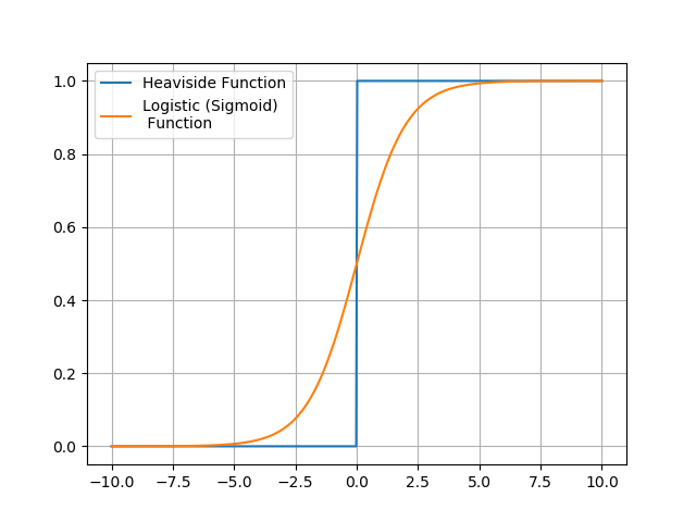
Note that the term “sigmoid function” refers to a family of s-shaped functions, of which the very popular logistic function is one of them. As such, it is common to see logistic and sigmoid used interchangeably, even though they are strictly not synonyms.
The logistic function performs better than the Heaviside function. In fact, machine learning using an artificial neuron that uses the logistic activation function is one and the same as logistic regression. Ha! You’ve probably run into that one before. Don’t feel left out if you haven’t though, because you’re just about to.
This is the equation for logistic regression:
\[\hat{y}=\frac{1}{1+e^{-\vec{z}}}\] \[\vec{z}\ =\ \vec{w}\mathbf{X}\ +\ b\]Where $ \hat{y} $ is the prediction or estimation (just another name for activation). It is a 1-by-$ m $ vector. It's not the unit vector for $ \vec{y} $.
And this is the equation for an artificial neuron with a logistic (sigmoid) activation function:
\[\vec{a}=\frac{1}{1+e^{-\vec{z}}}\] \[\vec{z}\ =\ \vec{w}\mathbf{X} + b\]As you can see, they are one and the same!
Also note that the perceptron, along with every other kind of artificial neuron, is an estimator just like other machine learning models (linear regression, etc.).
Besides the sigmoid and Heaviside functions, there are a plethora of other functions that have found great usefulness as activation functions. You can find a list of many other activation functions in this Wikipedia article. You should take note of the rectified linear function; any neuron using it is known as a rectified linear unit (ReLU). It’s the most popular activation function in deep learning as of 2020, and will likely remain so in the foreseeable future.
One more important mention is that the process of going from input data (\(\mathbf{X}\)) all the way to activation (essentially, the execution of an activation function) is called forward pass (or forward propagation in the context of neural networks), and this is the process we demonstrated above using the toy dataset. This distinguishes from the sequel process, known as backward pass, where we use the error between the activation (\(\vec{a}\)) and the ground truth (\(\vec{y}\)) to tune our parameters in such a way that the error decreases.
To tie things back to our toy dataset. If we used a logistic activation function instead of a Heaviside function, and trained our neuron for 2000 iterations, we obtain some values for the parameters that gives us the correct result 89% of the time. (We will later go over exactly what happens during “training”).
The parameters after training are:
\[\vec{w}=\left[\begin{matrix}0.33456&0.0206573\\\end{matrix}\right]\] \[b=-2.09148\]So, the optimized (trained) equation for our artificial neuron is:
\[\vec{z}\ =\ \left[\begin{matrix}0.33456&0.0206573\\\end{matrix}\right]\mathbf{X}\ +\left[\begin{matrix}-2.09148&-2.09148&-2.09148\\\end{matrix}\right]\] \[\vec{a}=\frac{1}{1+e^{-\vec{z}}}\]Where $ \mathbf{X} $ is an $ n $-by-$ m $ matrix that contains a batch of our dataset, and $ m $ is the number of datapoints in our batch, while $ n $ is the number of features in our dataset.
The above is the logistic artificial neuron that has learned the relationship hidden in our toy dataset, and you can randomly pick some datapoints in our dataset and verify the equation yourself. Roughly 9 out of 10 times, it should produce an activation that matches the ground truth (\(\vec{y}\)).
Note that the values for the parameters are not unique. A different set of values can still give us a comparable performance. We only discovered one of many possible sets of values that can give us good performance.
Loss function
In the section on estimators from part 1 of this blog series, I mentioned that it is imperative to expect an estimator (which is what an artificial neuron is) to have some level of error in its prediction, and our objective will be to minimize this error.
We described this error as:
\[\varepsilon =y-\hat{y}=f_{actual} \left( x \right) -f_{estim} \left( x \right)\]The above is actually one of the many ways to describe the error, and not rigorous enough. For example, it is missing an absolute value operator, else the sign of the error will change just based on how the operands of the subtraction are arranged:
\[y-\hat{y}\neq\hat{y}-y\]For instance, we know the difference between the natural numbers 5 and 3 is 2, but depending on how you rearrange the subtraction between them, we could end up with -2 instead, and we don’t want that to be happening, so we apply an absolute value operation and restate the error as:
\[\varepsilon=|y-\hat{y}|\]Now if we have a dataset made of more than one datapoint, we will have many errors, one for each datapoint. We need a way to aggregate all those individual errors into one big error value that we call the loss (or cost).
We achieve this by simply averaging all those errors to produce a quantity we call the mean absolute error:
\[Mean\ absolute\ error=Cost=\frac{1}{m} \cdot \sum _{j=0}^{m} \vert y_{j}-\hat{y}_{j} \vert =\frac{1}{m} \cdot \sum _{j=0}^{m} \varepsilon _{j}\]Where $ m $ is the number of datapoints in the batch of data. Note that $ \hat{y}_{j} $ is same as activation $ a_j $, and it is denoted here as such to show that it serves as an estimate for the ground truth $ y_j $.
The above equation happens to be just one of the many types of loss functions (a.k.a. cost function) in broad use today. They all have one thing in common: They produce a single scalar value (the loss or cost) that captures how well our network has learned the relationship between the features and the target for a given batch of a dataset.
Cost function vs loss function vs objective function
Some reserve the term loss function for when dealing with one datapoint and use cost function for the version that handles a batch of multiple datapoints. But such distinctions are purely up to personal taste, and it is common to see the two names used interchangeably.
|
We will introduce two other loss functions that are very widely used.
Mean squared error loss function, which is typically used for regression tasks:
\[Mean\ squared\ error:\ J=\frac{1}{m}\cdot\sum_{j}^{m}\left(y_j-a_j\right)^2\]You might have seen the above equation before if you’ve learned about linear regression.
Logistic loss function (also known as cross entropy loss or negative log-likelihoods), which is typically used for classification tasks, is:
\[Cross\ entropy\ loss:\ \ J = -\frac{1}{m}\cdot\sum_{j}^{m}{y_j\cdot\log{(a_j)}+(1-y_j)\cdot\log{({1-a}_j)}}=\frac{1}{m}\cdot\sum_{j=0}^{m}\varepsilon_j\]Note that the logarithm in the cross entropy loss is with base \(e\) (Euler’s number). In other words, it is a natural logarithm, which is sometimes abbreviated as \(\ln\) instead of \(\log\). In actuality, the logarithm can be in other bases, but that tends to make symbolically solving the cost derivatives more difficult. Also note that we are implicitly assuming that our ground truth is binary (i.e. only two classes and therefore binary classification).
What the cross entropy loss really says is that for class 0, the loss is:
\[-\log{({1-a}_j)}\]And for class 1, it is:
\[-\log{(a_j)}\]And the premise is that \(a_j\) is expected to always be between 0 and 1. This will be true if the activation function is logistic.
Loss as a function of parameters
Notice that all these loss functions have one thing in common, they are all functions of activation, which also makes them functions of the parameters:
\[Cost:\ \ J=f\left(\vec{a}\right)=f(\vec{w},b)\\]For instance, cross entropy loss function for a single datapoint can be recharacterized as follows:
\[Cross\ entropy\ loss=\ -\left(y\cdot\log{a})+(1-y)\cdot\log(1-a)\right)\] \[=-\left(data\cdot\log{\left(\frac{1}{1+e^{-z}}\right)}+\left(1-data\right)\cdot\log{\left(1-\frac{1}{1+e^{-z}}\right)}\right)\] \[=-\left(data\cdot\log{\left(\frac{1}{1+e^{\sum_{i=0}^{n}{w_i\ \cdot x_i}}}\right)}+\left(1-data\right)\cdot\log{\left(1-\frac{1}{1+e^{-\sum_{i=0}^{n}{w_i\ \cdot x_i}}}\right)}\right)\] \[=-\left(data+\left(1-\frac{1}{1+e^{\sum_{i=0}^{n}{w_i\ \cdot\ data}}}\right)\cdot\log{\left(1-\frac{1}{1+e^{-\sum_{i=0}^{n}{w_i\ \cdot\ data}}}\right)}\right)\\] \[=-\left(data\cdot\log{\left(\frac{1}{1+e^{\sum_{i=0}^{n}{w_i\ \cdot d a t a}}}\right)}+\left(1-data\right)\cdot\log{\left(1-\frac{1}{1+e^{-\sum_{i=0}^{n}{w_i\ \cdot data}}}\right)}\right)\\]In other words, the loss function can be described purely as a function of the parameters (\(\vec{w}\), \(b\)) and the data (\(\mathbf{X}\), \(\vec{y}\)). And since data is known, the only unknowns on the right-hand side of the equation are the parameters. Hence, it is really just a function of the parameters.
comments powered by Disqus