Catching AI with its pants down: Understand a Neural Network from Scratch
| We will strip the mighty, massively hyped, highly dignified AI of its cloths, and bring its innermost details down to earth! |
Prologue
This is part 5 of this blog series, Catching AI with its pants down. This blog series aims to explore the inner workings of neural networks and show how to build a standard feedforward neural network from scratch.
In this part, I will go over the mathematical underpinnings of a standard feedfoward neural network.
| Parts | The complete index for Catching AI with its pants down |
|---|---|
| Pant 1 | Some Musings About AI |
| Pant 2 | Understand an Artificial Neuron from Scratch |
| Pant 3 | Optimize an Artificial Neuron from Scratch |
| Pant 4 | Implement an Artificial Neuron from Scratch |
| Pant 5 | Understand a Neural Network from Scratch |
| Pant 6 | Optimize a Neural Network from Scratch |
| Pant 7 | Implement a Neural Network from Scratch |
| Pant 8 | Demonstration of the Models in Action |
Network of artificial neurons
A neural network is a network of artificial neurons. They are basically function approximators, and according to the universal approximation theorem, are capable of approximating continuous functions to any degree of accuracy. While that might sound very profound, the theorem doesn’t tell us how to optimize the neural network, so it is not a panacea.
We’ve seen how to build a single artificial neuron in part 1 to 4. We set up our equations entirely as equations of tensors, which makes transitioning to neural networks significantly easier.
In a neural network, the units (neurons) are stacked in layers, where outputs from the previous layer serve as the inputs to the next layer. Activations get propagated forward through the network, hence the name forward propagation (or simply forward pass). Errors get propagated backward through the network, hence the name backward propagation. The process of back propagation of errors and updating of weights are together commonly referred to as backward pass.
The input to the neural network is the data, and it is commonly referred to as the input layer. It may be the preprocessed data instead of the raw data. The input layer is not counted as the first layer of the network and is instead counted as the 0th layer if counted at all.
The last layer is known as the output layer and its output is the prediction or estimation. Every other layer in the network, which is any layer between the input and output layers, is called a hidden layer. This also means that the first hidden layer is also the first layer of the network.
For instance, a five-layer feedforward neural network has one input layer, four hidden layers and finally an output layer.
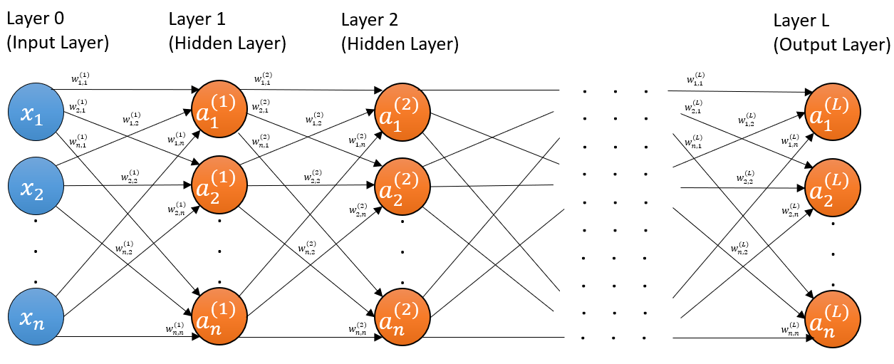
Neural networks come in an assortment of architectures. As an introduction, we are focusing on the standard feedforward neural network, also commonly referred to as multilayer perceptron, even though the neurons may not necessarily be the original perceptron with Heaviside activation function. The term feedforward indicates that our network has no loops or cycles; that is, the activations do no loop backward or within the layer but are always flowing forward. In contrast, there are architectures were activations cycle around, e.g. recurrent neural networks.
If you’re curious what other architecture exist out there, check out this beautiful article.
Forward propagation
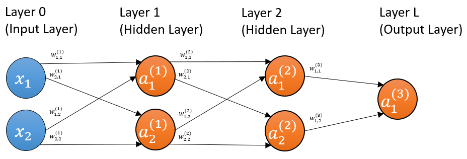
Now, let’s consider a three-layer multilayer perceptron, with two units in the first hidden layer, another two in the second hidden layer, and one unit in the output layer.
The notations being used here are as follows:
The activations are written as $ a_i^{(l)} $, where $ l $ is the serial number of the layer, and $ i $ is the serial number of the unit in the $ l $th layer. E.g. for the second unit of the second layer, it is $ a_2^{(2)} $.
The weight for each connection is denoted as $ w_{i,\ \ h}^{(l)} $, where $ l $ is the serial number of the layer (it always is), $ i $ is the serial number of the unit in the $ l $th layer, which is the destination of the connection, and $ h $ is the serial number of the unit in the $ (l-1) $th layer, which the origin of the connection.
As an example, $ w_{1,2}^{(3)} $ is the weight of the connection pointing from the 2nd unit of the 2nd layer (the unit with activation $ a_2^{(2)} $) to the 1st unit of the 3rd layer (the unit with activation $ a_1^{(3)} $).
Note that whenever we are focused on a specific layer, let's designate it as the current layer, it will be regarded as layer $ l $, and the layer before it will be layer $ l-1 $, while the layer after it will be layer $ l+1 $.
Just like in every article for this blog series, unless explicitly started otherwise, matrices (and higher-order tensors, which should be rare in this blog series) are denoted with boldfaced, non-italic, uppercase letters (e.g. $ \mathbf{A}^{(l)} $ for the matrix that holds all activations in layer $ l $); vectors are denoted with non-boldfaced, italic letters accented with a right arrow; and scalars are denoted with non-boldfaced, italic letters.
Other notations will be introduced along the way.
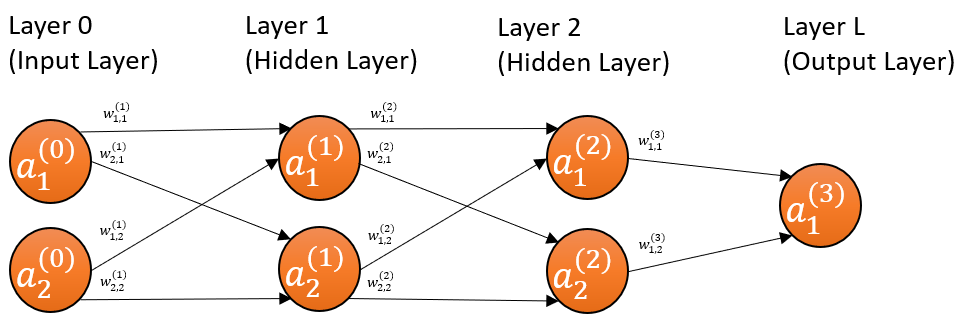
The input layer can be treated as the 0th layer, where \(x_i\) becomes denoted as \(a_i^{(0)}\). This means the number of features now becomes the number of units in the input layer. The bias node, which is usually never shown and always equal to 1, is treated as the 0th unit (node) in each layer .
Also, keep in mind that the diagrams do not reflect multiple examples (or datappoints or records). In otherwords, the diagrams are as if only one example is fed into the network per batch. Hence, \(a_2^{(2)}\) in the diagram is actually \({\vec{a}}_2^{(2)}\), and the latter reduces to the former for a batch size of one example.
Since we’ve thoroughly gone over how to mathematically characterize a single unit in part 2, we will use that as the springboard for delineating the three-layer network. Let’s focus on one of the units, say the second unit of the second layer.
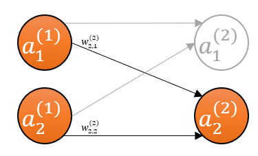
The inputs to the second unit of the second layer are the activations produced by the units of the first layer. We’ve seen exactly this in part 2, except that here our input to the second unit are activations (\(\mathbf{A}^{(1)}\)) instead of the data (\(\mathbf{X}\)).
Therefore, our equation of tensors is going to be:
\[{\vec{a}}_2^{(2)}=f\left({\vec{z}}_2^{(2)}\right)\] \[{\vec{z}}_2^{(2)}=\ {\vec{w}}_2^{(2)}\mathbf{A}^{(1)}\ +\ {\vec{b}}_2^{(2)}\]
Where $ {\vec{z}}_2^{(2)} $ and $ {\vec{a}}_2^{(2)} $, are the preactivations and activations of for the second unit in the second layer, and both have the same shape 1-by-$ m $, where $ m $ is the number of examples in the batch.
And $ {\vec{w}}_2^{(2)} $ contains the weights for the connections pointing to the second unit of the second layer, and it has the shape 1-by-$ n^{(2)} $, where $ n^{(2)} $ is the number of units in the second layer (layer 2).
$$
{\vec{w}}_2^{(2)}=\left[\begin{matrix}w_{2,\ 1}^{(2)}&w_{2,\ \ 2}^{(2)}\\\end{matrix}\right]
$$
And as in part 2, $ {\vec{b}}_2^{(2)} $ is fundamentally a scalar but gets broadcasted to match the shape of $ {\vec{z}}_2^{(2)} $ during computation.
And $ \mathbf{A}^{(1)} $ contains the activations from the first layer and has shape $ n^{(1)} $-by-$ m $, where $ n^{(1)} $ is the number of units in the first layer (layer 1).
This gives us a template to write out the equations for the other units in the network. For example, for the first unit in the second layer, we have:
\[{\vec{a}}_1^{(2)}=f\left({\vec{z}}_1^{(2)}\right)\] \[{\vec{z}}_1^{(2)}=\ {\vec{w}}_1^{(2)}\mathbf{A}^{(1)}\ +\ {\vec{b}}_1^{(2)}\]If we had more units in the second layer, the equation would be:
\[{\vec{a}}_i^{(2)}=f\left({\vec{z}}_i^{(2)}\right)\] \[{\vec{z}}_i^{(2)}=\ {\vec{w}}_i^{(2)}\mathbf{A}^{(1)}\ +\ {\vec{b}}_i^{(2)}\]Notice that we can now write the equations for the preactivations for the second layer:
\[{\vec{z}}_1^{(2)}=\ {\vec{w}}_1^{(2)}\mathbf{A}^{(1)}\ +\ {\vec{b}}_1^{(2)}\] \[z_2^{(2)}=\ {\vec{w}}_2^{(2)}\mathbf{A}^{(1)}\ +\ {\vec{b}}_2^{(2)}\] \[\vdots\] \[{\vec{z}}_{n^{(2)}}^{(2)}=\ {\vec{w}}_{n^{(2)}}^{(2)}\mathbf{A}^{(1)}\ +\ {\vec{b}}_{n^{(2)}}^{(2)}\]Just like in part 2, we can put the above system of equations into matrix format. One caveat is to remember that the terms in the above equations are themselves vectors and matrices, so we use relationship between matrix-matrix and vector-matrix multiplications:
\[\left[\begin{matrix}{\vec{z}}_1^{(2)}\\{\vec{z}}_2^{(2)}\\\vdots\\{\vec{z}}_{n^{(2)}}^{(2)}\\\end{matrix}\right]=\left[\begin{matrix}{\vec{w}}_1^{(2)}\mathbf{A}^{(1)}\\{\vec{w}}_2^{(2)}\mathbf{A}^{(1)}\\\vdots\\{\vec{w}}_{n^{(2)}}^{(2)}\mathbf{A}^{(1)}\\\end{matrix}\right]+\left[\begin{matrix}{\vec{b}}_1^{(2)}\\{\vec{b}}_2^{(2)}\\\vdots\\{\vec{b}}_{n^{(2)}}^{(2)}\\\end{matrix}\right]\] \[\mathbf{Z}^{(2)}=\mathbf{W}^{(2)}\mathbf{A}^{(1)}+\mathbf{B}^{(2)}\]Or in general, for a feedforward neural network:
\[\left[\begin{matrix}{\vec{z}}_1^{(l)}\\{\vec{z}}_2^{(l)}\\\vdots\\{\vec{z}}_{n^{(l)}}^{(l)}\\\end{matrix}\right]=\left[\begin{matrix}{\vec{w}}_1^{(l)}\mathbf{A}^{(l-1)}\\{\vec{w}}_2^{(l)}\mathbf{A}^{(l-1)}\\\vdots\\{\vec{w}}_{n^{(l)}}^{(l)}\mathbf{A}^{(l-1)}\\\end{matrix}\right]+\left[\begin{matrix}{\vec{b}}_1^{(l)}\\{\vec{b}}_2^{(l)}\\\vdots\\{\vec{b}}_{n^{(l)}}^{(l)}\\\end{matrix}\right]\] \[\mathbf{Z}^{(l)}=\mathbf{W}^{(l)}\mathbf{A}^{(l-1)}+\mathbf{B}^{(l)}\]Our preactivation tensor \(\mathbf{Z}^{(l)}\) is an \(n^{(l)}\)-by-\(m\) matrix of the form:
\[\mathbf{Z}^{(l)}=\left[\begin{matrix}{\vec{z}}_1^{(l)}\\{\vec{z}}_2^{(l)}\\\vdots\\{\vec{z}}_{n^{(l)}}^{(l)}\\\end{matrix}\right]=\left[\begin{matrix}z_{1,1}^{(l)}&z_{1,2}^{(l)}&\cdots&z_{1,m}^{(l)}\\z_{2,1}^{(l)}&z_{2,2}^{(l)}&\cdots&z_{2,m}^{(l)}\\\vdots&\vdots&\ddots&\vdots\\z_{n^{(l)},1}^{(l)}&z_{n^{(l)},2}^{(l)}&\cdots&z_{n^{(l)},m}^{(l)}\\\end{matrix}\right]\]The activation tensor \(\mathbf{A}^{(l-1)}\) is an \(n^{(l-1)}\)-by-\(m\) matrix. In general, the activation for any layer \(l\), denoted \(\mathbf{A}^{(l)}\), has the shape \(n^{(l)}\)-by-\(m\).
\[\mathbf{A}^{(l)}=\left[\begin{matrix}{\vec{a}}_1^{(l)}\\{\vec{a}}_2^{(l)}\\\vdots\\a_{n^{(l)}}^{(l)}\\\end{matrix}\right]=\left[\begin{matrix}a_{1,1}^{(l)}&a_{1,2}^{(l)}&\cdots&a_{1,m}^{(l)}\\a_{2,1}^{(l)}&a_{2,2}^{(l)}&\cdots&a_{2,m}^{(l)}\\\vdots&\vdots&\ddots&\vdots\\a_{n^{(l)},1}^{(l)}&a_{n^{(l)},2}^{(l)}&\cdots&a_{n^{(l)},m}^{(l)}\\\end{matrix}\right]\]The weight tensor \(\mathbf{W}^{(l)}\) is an \(n^{(l)}\)-by-\(n^{(l-1)}\) matrix, where \(n^{(l)}\) and \(n^{(l-1)}\) are number of units in the \(l\)th and \((l-1)\)th layers.
\[\mathbf{W}^{(l)}=\left[\begin{matrix}{\vec{w}}_1^{(l)}\\{\vec{w}}_2^{(l)}\\\vdots\\{\vec{w}}_{n^{(l)}}^{(l)}\\\end{matrix}\right]=\left[\begin{matrix}w_{1,1}^{(l)}&w_{1,2}^{(l)}&\cdots&w_{1,n^{(l-1)}}^{(l)}\\w_{2,1}^{(l)}&w_{2,2}^{(l)}&\cdots&z_{2,n^{(l-1)}}^{(l)}\\\vdots&\vdots&\ddots&\vdots\\w_{n^{(l)},1}^{(l)}&w_{n^{(l)},2}^{(l)}&\cdots&w_{n^{(l)},n^{(l-1)}}^{(l)}\\\end{matrix}\right]\]There is a reason why each of the above matrices is also presented as a column vector of row vectors. This kind of representation will come in very handy when we try to solve the cost gradients symbolically via back propagation.
And as you probably already expect, the full forward propagation equation for a feedforward neural network is:
\[\mathbf{Z}^{(l)}=\mathbf{W}^{(l)}\mathbf{A}^{(l-1)}+\mathbf{B}^{(l)}\] \[\mathbf{A}^{(l)}=f(\mathbf{Z}^{\left(l\right)})\]The way it works is we use our data (maybe after some preprocessing, like scaling the data, binning it, etc.) as the activations of the input layer \(\mathbf{A}^{(0)}\) to compute \(\mathbf{Z}^{(1)}\), and then use that to get \(\mathbf{A}^{(1)}\). Then we use \(\mathbf{A}^{(1)}\) to compute \(\mathbf{A}^{(2)}\). Then we use \(\mathbf{A}^{(2)}\) to compute \(\mathbf{Z}^{(3)}\) and subsequently \(\mathbf{A}^{(3)}\). We continue the pattern until we finally compute the activations of the output layer \(\mathbf{A}^{(L)}\) (where \(L\) is the serial number of the last layer).
It is quickly evident that the shape of \(\mathbf{A}^{(\mathbf{0})}\) is determined by the data, in particular by the number of features (\(\mathbf{X}\)), which becomes the number of units in the input layer. Similarly, the shape of \(\mathbf{A}^{(L)}\), and therefore number of units in the \(L\)th layer, is determined by the shape of the ground truth (\(y\)).
In the case of binary classification (i.e. the target only has two classes, e.g. male or female, malignant or benign, etc., which is encoded as 0 or 1), we know for certain that the ground truth will be a 1-by-\(m\) vector, but multi-class classification can lead to the ground truth being a higher order tensor.
How can our target (a.k.a. ground truth, dependent variable, response, etc.) be a higher order tensor (e.g. a matrix, order-three tensor, etc.)?
Say that our target contains nominal data. This means it won’t be proper to use a casual label encoding because we could encode the incorrect information.
|
In the analysis covered in this writeup, we will restrict our network to just binary classification or regression. The reason is to preclude the need for a softmax output layer (an output layer that’s using the softmax activation function), which is the preferred kind of output layer for dealing with multiclass classification problems. The reason we are excluding the softmax output layer is because it will add another stratum of complexity to the backprop calculations, and that’s best kept for a separate article as multiclass classification is a topic in its own right.
However, given the premise we decided to work with, we should’ve denoted the activation of the last layer as \(\vec{a}^{(L)}\) because we know it can only be a 1-by-\(m\) vector or a scalar (actually a 1-by-1 vector) if a batch of only 1 datapoint. But we will eschew all that and continue to denote it as \(\mathbf{A}^{(L)}\). This is purely for the sake of aesthetics and uniformity with the notations for the hidden layers, because the hidden layers are rightly denoted as \(\mathbf{A}^{(l)}\) as they are matrices (unless we limit each hidden layer to only one unit, which results in a vector).
comments powered by Disqus